3.4 Bayesian Model Comparison
Here we consider the problem of model selection from a Bayesian perspective. The Bayesian view of model comparison simply involves the use of probabilities to represent uncertainty in the choice of model. Suppose we wish to compare a set of $L$ models ${M_i}$ where $i = 1,…,L$. Here a model refers to a probability distribution over the observed data $D$. We shall suppose that the data is generated from one of these models but we are uncertain which one. Our uncertainty is expressed through a prior probability distribution $p(M_i)$. Given a training set $D$, we then wish to evaluate the posterior distribution
$$\begin{align} p(M_i|D) \propto p(M_i)p(D|M_i) \end{align}$$
The prior allows us to express a preference for different models. Let us simply assume that all the models are equally probable. Hence, the expression is mainly dependent on model evidence $p(D|M_i)$ which expresses the prefernce shown by the data for different models. The model evidence is sometimes called as the marginal likelihood because it can be viewed as the likelihood function over the space of the models. The ratio of model evidence $p(D|M_i)/p(D|M_j)$ for two models is known as Bayes factor. Once we know the posterior distribution over models, the predictive distribution is given as
$$\begin{align} p(t|X,D) = \sum_{i=1}^{L} p(t|X,M_i,D)p(M_i|D) \end{align}$$
This is an example of mixture distribution in which the overall predictive distribution is obtained by averaging the predictive distribution of individual models, weighted by the posterior distribution of these models. Another approach is to use the single most probable model alone to make the predictions. This is known as model selection. For a model governed by a set of parameters $W$, the model evidence is given as
$$\begin{align} p(D|M_i) = \int p(D|W,M_i)p(W|M_i)dW \end{align}$$
Let us consider the case of a model having a single parameter $w$. The posterior distribution is then proportional to (taking $p(M_i) = const$)
$$\begin{align} p(M_i|D) \propto p(M_i)p(D|M_i) \propto p(D|M_i) = \int p(D|w,M_i)p(w|M_i)dw \end{align}$$
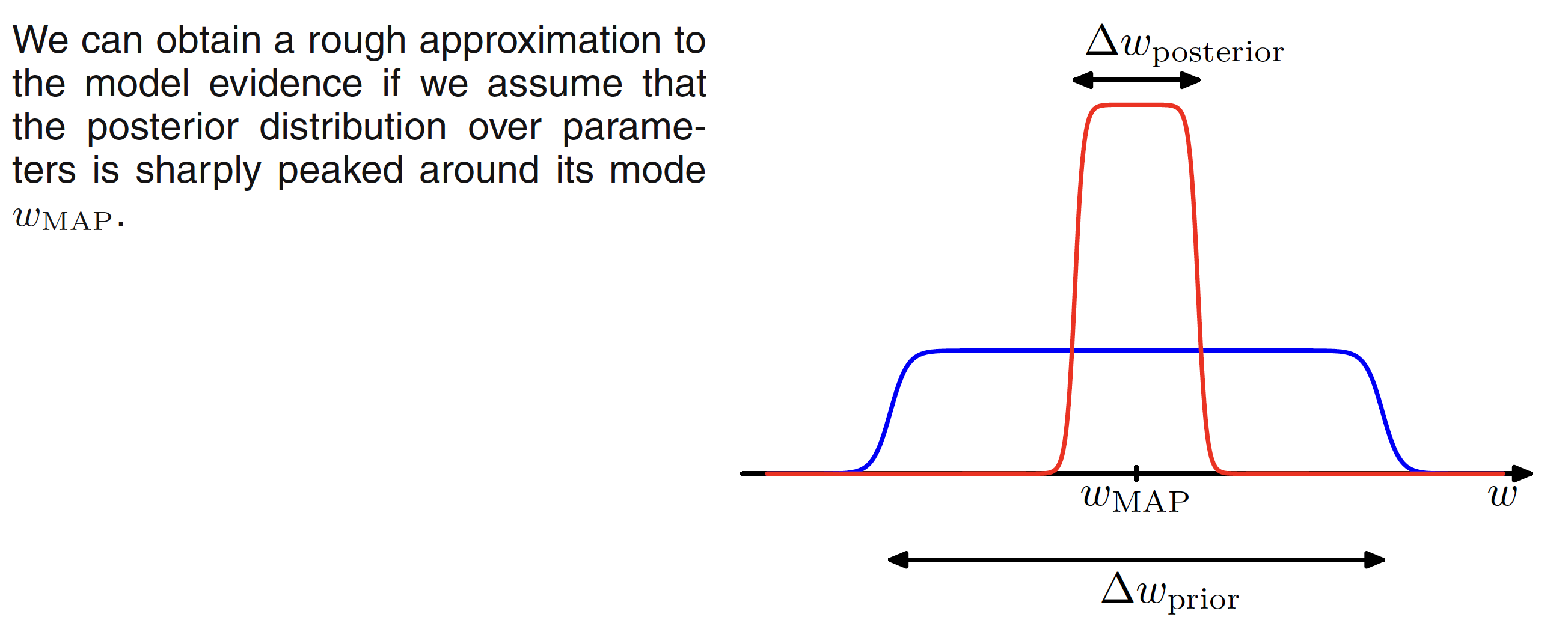
If we assume that the posterior distribution is sharply peaked around the most probable value $w_{MAP}$ with width $\Delta w_{posteriro}$, then the integral can be approximated by the value of the integrand at its maximum times the width of the peak. Assuming a flat prior with width $\Delta w_{prior}$ so that $p(w) = 1/\Delta w_{prior}$, then we have
$$\begin{align} p(D|M_i) = \int p(D|w,M_i)p(w|M_i)dw \simeq p(D|w_{MAP},M_i)\frac{\Delta w_{posterior}}{\Delta w_{prior}} \end{align}$$
Hence,
$$\begin{align} \ln p(D|M_i) \simeq \ln p(D|w_{MAP},M_i) + \ln \bigg(\frac{\Delta w_{posterior}}{\Delta w_{prior}}\bigg) \end{align}$$
Here, the first term represents how good fit the data is for a given model. The second term penalizes the model as per the complexity. As $\Delta w_{posterior} < \Delta w_{priro}$, this term is negative. It increases in magnitude as the ratio $\Delta w_{posterior}/\Delta w_{prior}$ gets smaller. This means that if the parameters are finely tuned to the data in the posterior distribution, the penalty term is large. This is illustrated in below figure
For a model having $M$ paramaters where all the parameters have the same ratio $\Delta w_{posterior}/\Delta w_{prior}$, we have
$$\begin{align} \ln p(D|M_i) \simeq \ln p(D|W_{MAP},M_i) + M\ln \bigg(\frac{\Delta w_{posterior}}{\Delta w_{prior}}\bigg) \end{align}$$
The complexity penalty increases as we increase the number of parameters in the model. For a more complex model, the first term will usually be small as a more complex model is a better fit to data but the second term will be large penalizing the model for complexity. The optimal model complexity will be determined by the maximum of this evidence which will be decided by the tradeoff between these two competing terms.