3.1.2 Geometry of Least Squares
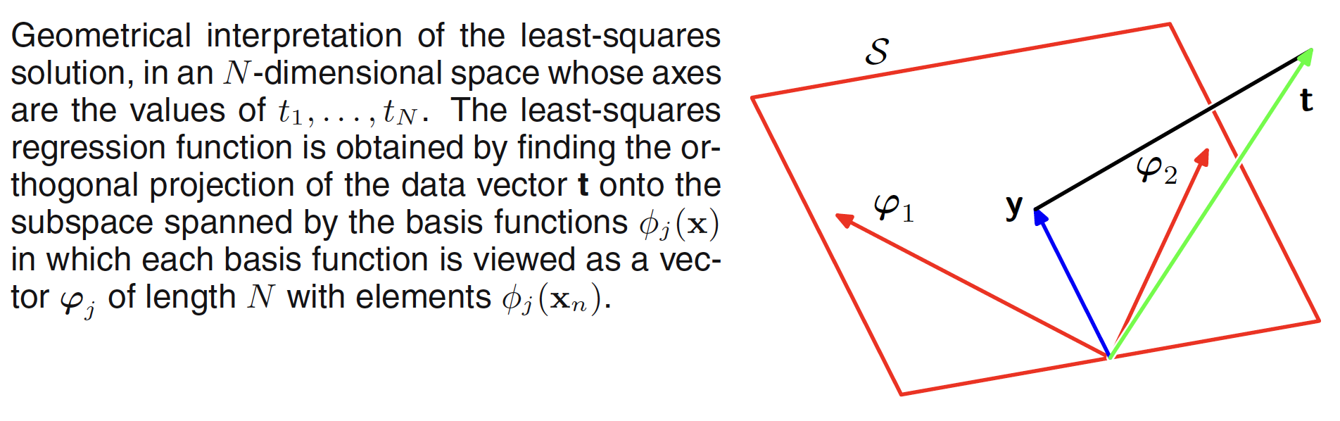
The least square problem can be geometrically interpreted as follows. Let the target veactor $t$ (having output for $N$ data points) spans a $N$-dimensional space. Each basis vector $\phi_j(X_n)$ will also be present in the same space. If the number $M$ of basis functions is smaller than the number of data points $N$, then the $M$ basis vectors will span a subspace $S$ of dimensionality $M$. The prediction $y(X,W)$ is the linear combination of basis vectors, it will lie in the subspace $S$. The least square solution corrsponds to the choice of $W$ for which $y(X,W)$ is closest to $t$. The interpretation is shown in the below figure.
3.1.3 Sequential Learning
In sequential learning, the data points are considered one at a time, and the model parameters updated after each such presentation. A sequential learning algorithm can be obtained by using the method of stochastic gradient descent or sequential gradient descent. If the error function is considerd as a sum over presented data points and is given as $E = \sum_n E_n$, the algorithm updates the parameter vector as
$$\begin{align} W^{(\tau+1)} = W^{(\tau)} - \eta \nabla E_n \end{align}$$
where $\tau$ denotes the iteration number and $\eta$ is the learning parameter. The value of $W$ is initialized to some starting vector $W^{(0)}$. For sum-of-squares error function, the equation reduces to
$$\begin{align} W^{(\tau+1)} = W^{(\tau)} + \eta(t_n - W^{(\tau)T}\phi_n)\phi_n \end{align}$$
where $\phi_n = \phi(X_n)$. This is known as least-mean-squares (LMS) algorithm.
3.1.4 Regularized Least Squares
To reduce overfitting, a regularization term can be added to the error function. With the regularization term added, the error function is given as
$$\begin{align} E_D(W) + \lambda E_W(W) \end{align}$$
where $\lambda$ is the regularization term which controls the data dependent error $E_D(W)$ and the regularization term $E_W(W)$. One of the examples of regularization is $L2$ regularization, given as
$$\begin{align} E_W(W) = \frac{1}{2}W^TW \end{align}$$
The total error function with sum-of-squares error will be
$$\begin{align} E_W(W) = \frac{1}{2}\sum_{n=1}^{N}\bigg(t_n - W^T\phi(X_n)\bigg)^2 + \frac{\lambda}{2}W^TW \end{align}$$
This particular choice of regularizer is also called as weight decay or parameter shrinkage method. As the error function is still a quadratic form of $W$, it can be minimized in a closed form. The regularized weight function is
$$\begin{align} W_{ML} = (\lambda I + \phi^T\phi)^{-1}\phi^Tt \end{align}$$
which is an extension to the least-square-solution. A more general regularized error term can be given as
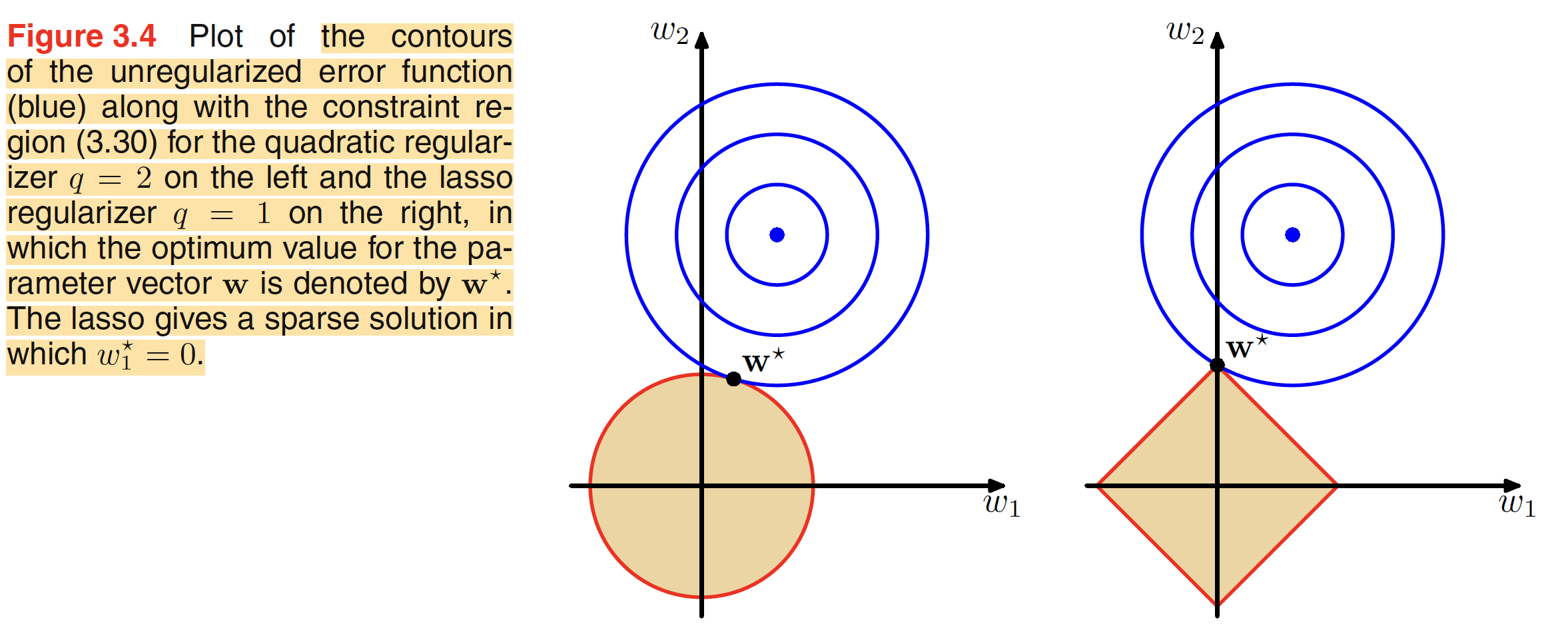
$$\begin{align} E_W(W) = \frac{1}{2}\sum_{n=1}^{N}\bigg(t_n - W^T\phi(X_n)\bigg)^2 + \frac{\lambda}{2}\sum_{j=1}^{M}|W_j|^q \end{align}$$
where $q=2$, corresonds to the quadratic or $L2$ regularizer. When $q=1$, we have lasso model. In this, when $\lambda$ is sufficiently large, some of the weight terms can go to $0$. The above minimization problem can be viewed as minimizing the unregularized sum-of-squares with the constraint
$$\begin{align} \sum_{j=1}^{M}|W_j|^q \leq \eta \end{align}$$
and can be solved using Lagrange Multiplier approach. A geomrtrical interpretation of regularization is shown in below figure.
3.1.5 Multiple Outputs
In some application, we may wish to predict $K>1$ target variable for one data point. One way to handle this is using treat each target variable as independent regression problem where we have to use different set of basis function for each regression problem. Another approach is to use same set of basis functions to model all the components of the target variable. The prediction can be given as
$$\begin{align} y(X,W) = W^T\phi(X) \end{align}$$
The above equation is same as the one for a single target variable case with only difference being is in the single target variable case, $W$ is a $M-$dimensional vector but here it is a $M \times K$ matrix of parameters. The solution for the parameter matrix is given as
$$\begin{align} W_{ML} = (\phi^T\phi)^{-1}\phi^TT \end{align}$$