2.5 Nonparametric Methods
Till now to model the data, we have choosen distributions which are governed by some fixed small number of parameters. This is called as parametric approach to density modeling. The chosen density might be a poor model of the distribution that generates the data, which can result in poor predictive performance. In nonparametric approach, we make fewer assumptions about the form of distribution.
One common nonparametric approach is histogram density models. In this approach, we partition $x$ into bins of width $\Delta_i$ and then count the number of observations falling in the bins (denoted as $n_i$). To have the normalized probability distribution, we can calculate the probability for eac bin as
$$\begin{align} p_i = \frac{n_i}{N\Delta_i} \end{align}$$
where $N$ is the total number of observations and $\int p(x)dx = 1$. An illustration of histogram density model is shown below.
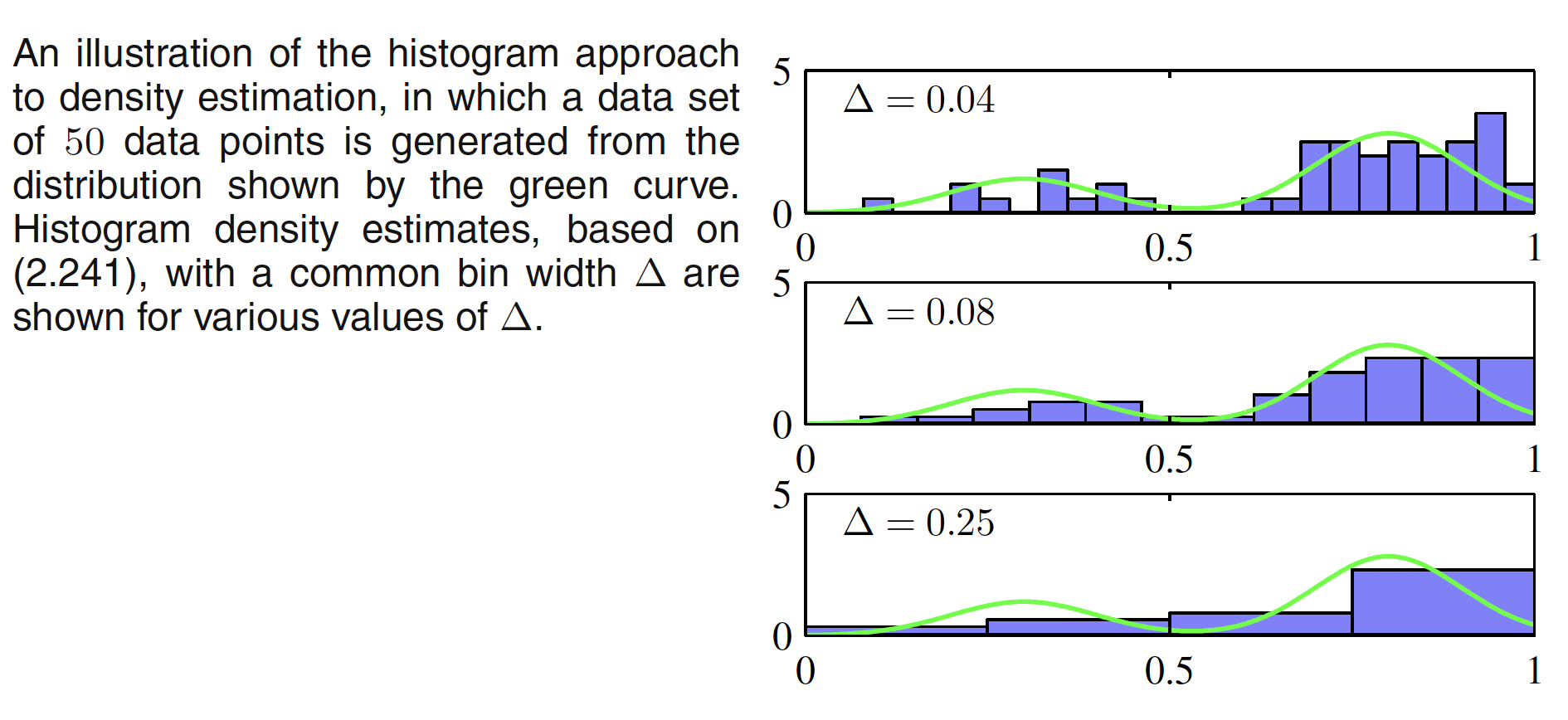
For smaller value of $\Delta$, the resulting density model is spiky with a lot of structure that is not present in the underlying distribution. For larger $\Delta$, the resultant model is too smooth and misses the bimodal property of underlying distribution. The best result is obtained by some intermediate value of $\Delta$. One of the advantage of histogram density models is that once the histogram has been computed, we can discard the dataset. One of the obvious disadvantage of this model is that the estimated densities have discontinuties due to the bin edges. Another major limitation of the histogram approach is its scaling with dimensionality. If we divide each variable in a $D$-dimensional space into $M$ bins, then the total number of bins will be $M^D$. This exponential scaling with $D$ is an example of the curse of dimensionality.
Histogram density estimation approach teaches us following important technique though:
-
First, to estimate the probability density at a particular location, we should consider the data points that lie within some local neighbourhood of that point. Note that the concept of locality requires that we assume some form of distance measure, and here we have been assuming Euclidean distance.
-
Second, the neighbourhood property was defined by the bins, and there is a natural ‘smoothing’ parameter describing the spatial extent of the local region, in this case the bin width. The value of the smoothing parameter should be neither too large nor too small in order to obtain good results.
2.5.1 Kernel Density Estimators
Let us suppose that observations are being drawn from some unknown probability density $p(x)$ in some $D$-dimensional space. From our earlier discussion of locality, let us consider some small region $R$ containing $x$. The probability mass associated with this region is given by
$$\begin{align} P = \int_{R} p(x)dx \end{align}$$
Now suppose that we have collected a data set comprising $N$ observations drawn from $p(x)$. Because each data point has a probability $P$ of falling within $R$, the total number $K$ of points that lie inside $R$ will be distributed according to the binomial distribution
$$\begin{align} Bin(K|N,P) = \frac{N!}{K!(N-K)!}P^K(1-P)^{1-K} \end{align}$$
The mean fraction of points falling inside this region is $E[K/N]=P$ with a variance of $Var[K/N]=P(1-P)/N$. As $N \to \infty$, the distributio will be sharply peaked around the mean and hence $K \simeq NP$. For a sufficiently small region $R$ with volume $V$, the probability density $p(x)$ is roughly constant over the region and then, we have
$$\begin{align} P \simeq p(x)V \end{align}$$
From the above two equations, we get the density estimate as
$$\begin{align} p(x) = \frac{K}{NV} \end{align}$$
We can exploit this equation in two ways:
-
We can fix $K$ and determine the value of $V$ from the data. This is called K-nearest-neighbour technique.
-
We can fix $V$ and determine $K$ from the data. This is called as kernal approach.
For the kernal approach, let $R$ be the small hypercube centred at $x$ at which we have to determine the density. A unit cube centred around the origin can be given as
$$\begin{align} k(u)= \begin{cases} 1, & |u_i| \leq 1/2;i=1,2,…,D\ 0, & \text{otherwise} \end{cases} \end{align}$$
$k(u)$ is an example of kernel function. For a datapoint $x_n$ the quantity $k((x-x_n)/h)$ will be $1$ if it lies inside the cube of side $h$ centred on $x$ and $0$ otherwise. The total number of datapoints lying inside this cube will be
$$\begin{align} K = \sum_{n=1}^{N} k\bigg( \frac{x-x_n}{h} \bigg) \end{align}$$
The estimated density is given as
$$\begin{align} p(x) = \frac{1}{N}\sum_{n=1}^{N} \frac{1}{h^D} k\bigg( \frac{x-x_n}{h} \bigg) \end{align}$$
as the volume $V=h^D$. Kernel density estimator suffers from the same problem of discontinuties at the boundries. A smoother density model is obtained when a smoother kernel function is used. Gaussian Kernel is one of the choices, which gives rise to the follwing density model
$$\begin{align} p(x) = \frac{1}{N}\sum_{n=1}^{N}\frac{1}{(2\pi h^2)^{1/2}} exp\bigg[ - \frac{||x-x_n||^2}{2h^2}\bigg] \end{align}$$
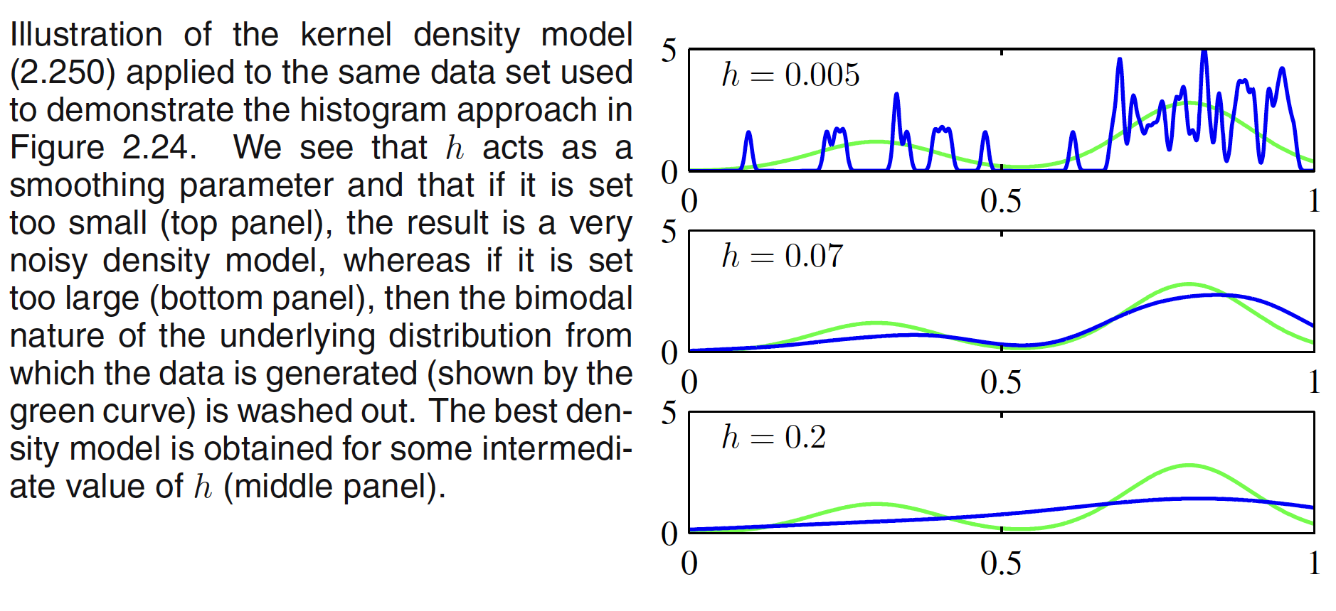
where $h$ represents the standard deviation of the Gaussian components. Thus our density model is obtained by placing a Gaussian over each data point and then adding up the contributions over the whole data set, and then dividing by $N$ so that the density is correctly normalized. Tha result of Gaussian kernel density estimation is shown below. It can be seen that the optimization of $h$ determines how fit the density model is to the dataset.
It should be noted that any kernel function $k(u)$ can be chosen for the density estimation task subject to the conditions
$$\begin{align} k(u) \geq 0 \end{align}$$
$$\begin{align} \int k(u) du = 1 \end{align}$$
2.5.2 Nearest-neighbours Method
One of the drawbacks of kernel approach is that $h$ is fixed irrespective of data density in the regions. In regions of high data density, a large value of $h$ may lead to over-smoothing and a washing out of structure that might otherwise be extracted from the data. However, reducing $h$ may lead to noisy estimates elsewhere in data space where the density is smaller. In Nearest-neighbours Method, we fix the $K$ and determine the value of $V$ from the data. To do this, we consider a small sphere centred at $x$ at which we have to estimate the density $p(x)$ and we allow the sphere to grow until it contains precisely $K$ points. The density is then given by the following equation with $V$ set as the volume of the sphere.
$$\begin{align} p(x) = \frac{K}{NV} \end{align}$$
The value of $K$ now governs the degree of smoothing and that again there is an optimum choice for $K$ that is neither too large nor too small. Note that the model produced by $K$ nearest neighbours is not a true density model because the integral over all space diverges.
The $K$-nearest-neighbour technique for density estimation can be extended to the problem of classification. Let us suppose that we have a data set comprising $N_k$ points in class $C_k$ with $N$ points in total, so that $\sum_{k}N_k = N$. If we wish to classify a new point $x$, we draw a sphere centred on $x$ containing precisely $K$ points irrespective of their class. Suppose this sphere has volume $V$ and contains $K_k$ points of class $C_k$. The estimate of density associated with each class is given as
$$\begin{align} p(x|C_k) = \frac{K_k}{N_kV} \end{align}$$
The unconditional density is given as
$$\begin{align} p(x) = \frac{K}{NV} \end{align}$$
and the class priors as
$$\begin{align} p(C_k) = \frac{N_k}{N} \end{align}$$
From Bayes’ theorem, we get
$$\begin{align} p(C_k|x) = \frac{p(X|C_k)p(C_k)}{p(x)} = \frac{K_k}{K} \end{align}$$
The probability of misclassification can be minimized by assigning the point to the class with highest posterior probability (i.e. the one which has the largest value of $K_k/K$). Here $K$ controls the degree of smoothness. It should be noted that these nonparametric methods are still severely limited.