Introduction :
Naive Bayes is an extremely fast classification algorithm which uses Bayes Theorem as its basic building block. It assumes that the features or predictors in the dataset are independent.
The Bayes theorem is given as:
$$P(c|X) = \frac{P(c)P(X|c)}{P(X)}$$
where $c$ denotes a class label and $X$ is the predictor. The probabilities $P(c)$ and $P(X)$ are the prior probabilities of the class and the predictor. $P(X|c)$ is the prior probability or likelihood of observing a feature $X$ given class $c$. $P(c|X)$ is the posterior probability of the class $c$ given a feature $X$. Hence, the posterior probability of a class $c$ givena a feature $X$ can be found using different prior probabilities and likelihood which can be obtained from the existing dataset. In the plain english, the Bayes theorem can be stated as:
$$posterior = \frac{prior \times likelihood}{evidence}$$
For picking up the most probable class based of different posterior probabilities, we can simply use a decision rule that picks up the class or hypothesis which is most probable. This is known as maximum a posteriori or MAP decision rule.
Example :
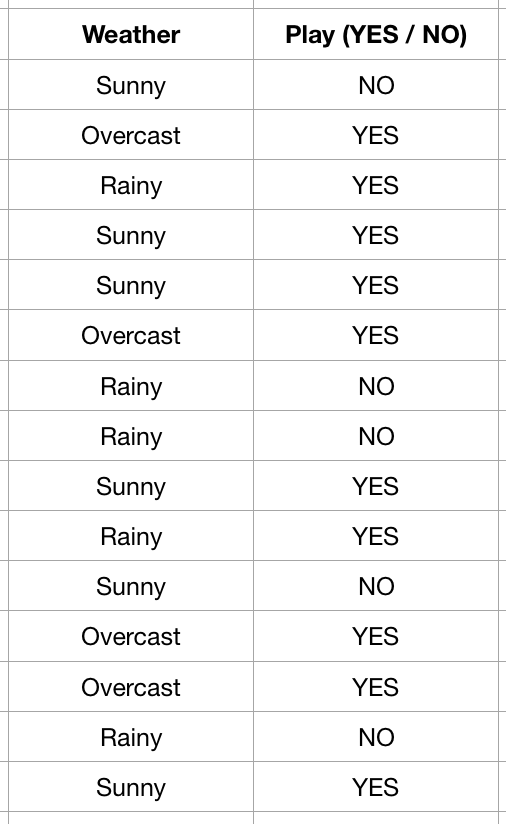
Let us look at an example. Given a dataset having the weather conditions and whether the players will play the golf or not based on these conditions, our task is to predict or classify that whether a player will play or not in a particular weather. The dataset is shown below.
As explained, it consists of the information that whether a player plays golf or not depending on the weather condition. A frequecy table, which can be further used to obtain prior proababilities and likelihood is shown below.
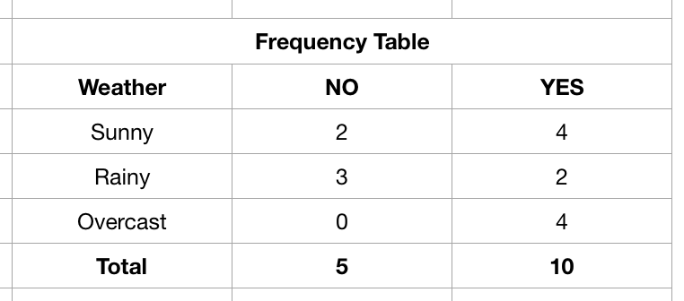
Let us ask ourselves a simple question: “Whether a player will play or not in a Sunny weather?". First of all we need to calculate the prior probabilities. The prior probabilities of classes and features are given as: $P(YES) = \frac{10}{15} = \frac{2}{3}$, $P(NO) = \frac{5}{15} = \frac{1}{3}$, $P(Sunny) = \frac{6}{15} = \frac{2}{5}$, $P(Rainy) = \frac{5}{15} = \frac{1}{3}$ and $P(Overcast) = \frac{4}{15}$. Now, we need to evaluate $P(YES|Sunny)$. For this, we have to find the likelihood $P(Sunny | YES)$ which is equal to $\frac{4}{10} = \frac{2}{5}$. Hence, the posterior probability can be evaluated as:
$$P(YES | Sunny) = \frac{P(YES)P(Sunny | YES)}{P(Sunny)} = \frac{\frac{2}{3} \times \frac{2}{5}}{\frac{2}{5}} = \frac{2}{3}$$
As there are only two probable classes, we can say that $P(NO | Sunny) = 1 - P(YES | Sunny) = \frac{1}{3}$. Hence the odds of a player playing golf on a suuny day is $\frac{\frac{2}{3}}{\frac{1}{3}} = 2$.
Advantage, Disadvantage and other concerns :
Naive Bayes is a powerful and easy to implement classifier. One major advantage of Naive Bayes is that it only requires a small number of training data to estimate the parameters necessary for classification. It also has an advantage of performing well in the case of multi-class classifier. If the assumption of independece holds, it can outperform various other classification algorithm such as logistic regression and LDA.
As we need to know the prior probabilities (distribution) and likelihoods in order to obtain the classification results, in the case of numeric features, we need to guess its prior distribution. One common way to implement the Naive Bayes in the case of numeric variables is to assume the prior distribution as Gaussian. Sometimes this assumption can be a bit too strong and hence Naive Bayes’ performance is comparatively better when the features are categorical.
Naive Bayes often suffers from the problem of missing category. When a feature has a category in the test data which is missing in the training set, the model makes a probability estimate of 0 and hence the classification algorithm will fail. This problem can be overcomed by incorporating a small-sample correction called pseudocount in all probability estimates and hence making them non-zeor. This way of regularizing naive Bayes is called as Laplace smoothing when the pseudocount is 1.
Naive Bayes for quantitative variable :
When dealing with continuous variable, one approach is to discretize the features by a simple process of binning. Another approach is to make an assumption that the continuous value associated with each class follows a Gaussian distribution. For this, we need to estimate the parameters $\mu_k$ and $\sigma_k^2$ (mean and variance) of every feature for each of the associated class labels. Then, the probability distribution or likelihood of a feature having a particular value can be calculated by plugging the value in the equation of a Normal distribution having parameters $\mu_k$ and $\sigma_k^2$.
#### Reference :https://en.wikipedia.org/wiki/Naive_Bayes_classifier
https://www.analyticsvidhya.com/blog/2017/09/naive-bayes-explained/