6.8 Exercises
Conceptual
Q1. We perform best subset, forward stepwise, and backward stepwise selection on a single data set. For each approach, we obtain p + 1 models, containing 0, 1, 2, . . . , p predictors. Explain your answers:
(a) Which of the three models with k predictors has the smallest training RSS?
Sol: Training RSS is minimum for best subset selection.
(b) Which of the three models with k predictors has the smallest test RSS?
Sol: The test RSS can not be predicted accurately based on the training procedure but as best subset selection takes into account all the possible models, there is a more chance of its getting the best test RSS.
(c) True or False:
-
The predictors in the k-variable model identified by forward stepwise are a subset of the predictors in the (k+1)-variable model identified by forward stepwise selection: True
-
The predictors in the k-variable model identified by backward stepwise are a subset of the predictors in the (k + 1)- variable model identified by backward stepwise selection.: True
-
The predictors in the k-variable model identified by backward stepwise are a subset of the predictors in the (k + 1)- variable model identified by forward stepwise selection.: False
-
The predictors in the k-variable model identified by forward stepwise are a subset of the predictors in the (k+1)-variable model identified by backward stepwise selection.: False
-
The predictors in the k-variable model identified by best subset are a subset of the predictors in the (k + 1)-variable model identified by best subset selection.: False
Q2. For parts (a) through (c), indicate which of i. through iv. is correct. Justify your answer.
(a) The lasso, relative to least squares, is:
i. More flexible and hence will give improved prediction accuracy when its increase in bias is less than its decrease in variance.: False
ii. More flexible and hence will give improved prediction accuracy when its increase in variance is less than its decrease in bias.: False
iii. Less flexible and hence will give improved prediction accuracy when its increase in bias is less than its decrease in variance.: True
iv. Less flexible and hence will give improved prediction accuracy when its increase in variance is less than its decrease in bias.: False, as lasso will decrease the variance and increase the bias.
(b) Repeat (a) for ridge regression relative to least squares.
Sol: Less flexible and hence will give improved prediction accuracy when its increase in bias is less than its decrease in variance.
(c) Repeat (a) for non-linear methods relative to least squares.
Sol: More flexible and hence will give improved prediction accuracy when its increase in variance is less than its decrease in bias.
Q3. Suppose we estimate the regression coefficients in a linear regression model by minimizing
$$minimize _{\beta}\bigg [ \sum _{i=1}^{n} \bigg( y_i - (\beta_0 + \sum _{j=1}^{p} \beta_j x _{ij})\bigg)^2 \bigg] \ \ \ subject \ to \ \sum _{j=1}^{p} |\beta_j| \leq s$$
for a particular value of s. For parts (a) through (e), indicate which of i. through v. is correct. Justify your answer.
(a) As we increase s from 0, the training RSS will:
Sol: Steadily decrease, as training RSS will become better and better as we will keep on adding new parameters.
(b) Repeat (a) for test RSS.
Sol: Decrease initially, and then eventually start increasing in a U shape.
(c) Repeat (a) for variance.
Sol: Steadily increase.
(d) Repeat (a) for (squared) bias.
Sol: Steadily decrease.
(e) Repeat (a) for the irreducible error.
Sol: Remain constant.
Q4. Suppose we estimate the regression coefficients in a linear regression model by minimizing
$$minimize _{\beta}\bigg [ \sum _{i=1}^{n} \bigg( y_i - (\beta_0 + \sum _{j=1}^{p} \beta_j x _{ij})\bigg)^2 \bigg] \ \ \ subject \ to \ \sum _{j=1}^{p} \beta_j^2 \leq s$$
for a particular value of λ. For parts (a) through (e), indicate which of i. through v. is correct. Justify your answer.
(a) As we increase λ from 0, the training RSS will:
Sol: Steadily increase.
(b) Repeat (a) for test RSS.
Sol: Decrease initially, and then eventually start increasing in a U shape.
(c) Repeat (a) for variance.
Sol: Steadily decrease.
(d) Repeat (a) for (squared) bias.
Sol: Steadily increase.
(e) Repeat (a) for the irreducible error.
Sol: Remain constant.
Q5. It is well-known that ridge regression tends to give similar coefficient values to correlated variables, whereas the lasso may give quite different coefficient values to correlated variables. We will now explore this property in a very simple setting.
Suppose that n = 2, p = 2, $x _{11} = x _{12}, x _{21} = x _{22}$. Furthermore, suppose that $y_1+y_2 = 0$ and $x _{11}+x _{21} = 0$ and $x _{12} + x _{22} = 0$, so that the estimate for the intercept in a least squares, ridge regression, or lasso model is zero: $\widehat{\beta_0}$ = 0.
The estimate of the intercept is 0, as $y_1+y_2 = 0$.
(a) Write out the ridge regression optimization problem in this setting.
Sol: Let the estimates of coefficients be $\beta_1$ and $\beta_2$. In case of ridge regression, we need to optimize:
$$(y_1 - \beta_1 X _{11} - \beta_2 X _{12})^2 + (y_2 - \beta_1 X _{21}- \beta_2 X _{22})^2 + \lambda(\beta_1^2 + \beta_2^2 )$$
(b) Argue that in this setting, the ridge coefficient estimates satisfy $\beta_1 = \beta_2$.
Sol: For the optimization, we need to take the partial derivative of the above expression with respect to $\beta_1$ and $\beta_2$ and evaluate it to 0. Replacing $X _{11} = X _{12} = -X _{21} = -X _{22} = a$ and $y_1 = -y_2 = b$ the equation reduces to:
$$2[b - a(\beta_1 + \beta_2)]^2 + \lambda(\beta_1^2 + \beta_2^2)$$
Taking partial derivatives with respect to $\beta_1$ and $\beta_2$ and setting them to 0, we get:
$$2\lambda \beta_1 = 4a[b - a(\beta_1 + \beta_2)]$$
$$2\lambda \beta_2 = 4a[b - a(\beta_1 + \beta_2)]$$
As the RHS of both the equations are same, we get $\beta_1 = \beta_2$.
(c) Write out the lasso optimization problem in this setting.
Sol: The lasso optimaization problem is:
$$(y_1 - \beta_1 X _{11} - \beta_2 X _{12})^2 + (y_2 - \beta_1 X _{21}- \beta_2 X _{22})^2 + \lambda(|\beta_1| + |\beta_2| )$$
(d) Argue that in this setting, the lasso coefficients $\beta_1$ and $\beta_2$ are not unique—in other words, there are many possible solutions to the optimization problem in (c). Describe these solutions.
Sol: Replacing the values as discussed above, we get the optimization problem:
$$2[b - a(\beta_1 + \beta_2)]^2 + \lambda(|\beta_1| + |\beta_2|)$$
Taking partial derivatives with respect to $\beta_1$ and $\beta_2$ and setting them to 0, we get:
$$4a[b - a(\beta_1 + \beta_2)] = \pm \lambda$$
The sign of RHS depends on the sign of $\beta$s. If $\beta_1$ and $\beta_2$ are positive, sign is +, if they are negative sign is -. This equation represents the boundary of the lasso constraint and hence the lasso optimization problem has many possible solutions.
Q6. We will now explore (6.12) and (6.13) further. These equation represents the special case for the lasso and ridge regression. In this case $n=p$ and all the diagonal elements of data set is 1 and the non-diagonal elements are 0. In this case the optimization problem for ridge regression and the lasso reduces to:
$$\sum _{j=1}^{p}(y_j - \beta_j)^2 + \lambda \sum _{j=1}^{p} \beta_j^2$$
$$\sum _{j=1}^{p}(y_j - \beta_j)^2 + \lambda \sum _{j=1}^{p} |\beta_j|$$
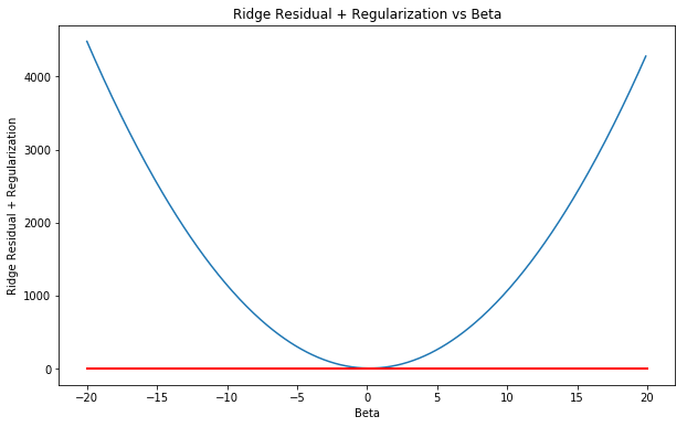
(a) Consider (6.12) with p = 1. For some choice of $y_1$ and λ > 0, plot (6.12) as a function of $\beta_1$. Your plot should confirm that (6.12) is solved by (6.14).
Sol: Equation (6.14) is given as:
$$\widehat{\beta_j}^R = \frac{y_j}{1 + \lambda}$$
Let $y_1 = 5, \lambda = 10$. The plot is shown below. The red line shows the plot of the solution for the ridge regression in this case. It is evident that the line crosses through the minimum error value.
import numpy as np
import matplotlib.pyplot as plt

y = 2
_lambda = 10
print(y/(1 + _lambda))
beta = np.arange(-20,20, 0.1)
ridge  = (y-beta)**2 + _lambda*(beta)**2

fig = plt.figure(figsize=(10, 6))
ax = fig.add_subplot(111)

plt.plot(beta, ridge)
plt.plot([-20, 20], [(y/(1 + _lambda)), (y/(1 + _lambda))], 'k-', color='r', lw=2) # Plot of solution

ax.set_xlabel('Beta')
ax.set_ylabel('Ridge Residual + Regularization')
ax.set_title('Ridge Residual + Regularization vs Beta')

plt.show()
0.18181818181818182
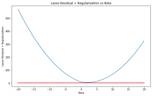
(b) Consider (6.13) with p = 1. For some choice of $y_1$ and λ > 0, plot (6.13) as a function of $\beta_1$. Your plot should confirm that (6.13) is solved by (6.15).
Sol: Equation (6.15) is given as:
$$ \begin{equation*} \beta_j^L= \left{ \begin{array}{@{}ll@{}} y_j - \lambda/2, & \text{if}\ y_j > \lambda/2 \ y_j + \lambda/2, & \text{if}\ y_j < -\lambda/2 \ 1, & \text{if} \ |y_j| \leq \lambda/2 \end{array}\right. \end{equation*} $$
The plot is shown below. The red line shows the plot of the solution for the lasso in this case (solution is $y_j - \lambda/2$). It is evident that the line crosses through the minimum error value.
y= 3
_lambda = 2
lasso  = (y-beta)**2 + _lambda*np.absolute(beta)

fig = plt.figure(figsize=(10, 6))
ax = fig.add_subplot(111)

plt.plot(beta, lasso)
plt.plot([-20, 20], [y-_lambda/2, y-_lambda/2], 'k-', color='r', lw=2) # Plot of solution

ax.set_xlabel('Beta')
ax.set_ylabel('Lasso Residual + Regularization')
ax.set_title('Lasso Residual + Regularization vs Beta')

plt.show()