6.2 Shrinkage Methods
As an alternative to subset selection methods, a model containing all the $p$ predictors can be fit using a technique that constrains or regularizes the coefficient estimates (or shrinks the coefficeint estimates towards 0). Two best known techniques for shrinking the coefficient estimates towards 0 are: ridge regression and the lasso.
6.2.1 Ridge Regression
In a least squares fitting, the parameters of the model is estimated by minimizing
$$RSS = \sum _{i=1}^{n} \bigg( y_i - (\beta_0 + \sum _{j=1}^{p} \beta_j x _{ij})\bigg)^2$$
In ridge regression, coefficients are estimated by minimizing the following term instead:
$$RSS + \lambda \sum _{j=1}^{p} \beta_j^2 = \sum _{i=1}^{n} \bigg( y_i - (\beta_0 + \sum _{j=1}^{p} \beta_j x _{ij})\bigg)^2 + \lambda \sum _{j=1}^{p} \beta_j^2$$
where $\lambda \geq 0$ is called as the tuning parameter and is determined separately. In ridge regression, the model fits the data well by minimizing RSS and shrinking penalty ($\lambda \sum _{j=1}^{p} \beta_j^2$). Shrinking penalty will be small when $\beta_i$s will be close to 0 and hence minimizing this has the effect of shrinking the coefficient estimates towards 0. When the tuning parameter $\lambda$ is 0, ridge regression will give the least squares estimates. For the larger value of $\lambda$, the impact of shrinkage penalty increases and hence the coefficient estimates approach closer to 0. We can generate different sets of coefficient estimates for different values of $\lambda$. The best estimate can be chosen using several cross-validation methods. It is to be noted that the shrinkage penalty is not applied to the intercept.
When value of $\lambda$ is very large, all the ridge regression coefficients approach 0, giving us the null model (model whic contain only intercept and no predictors). In aggregate, the ridge regression coefficients tend to decrease as $\lambda$ increases but some of the individual coefficients may increase. This phenomenon is shown in the left hand side figure below.
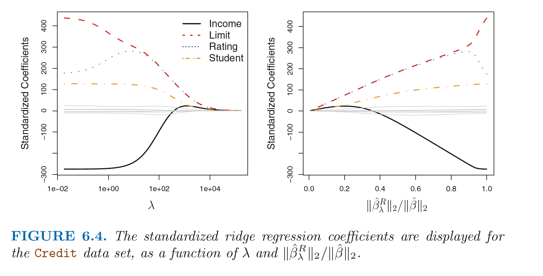
Instead we can plot the ridge coefficients against the ratio of l$_2$ norms of the ridge coefficients vector and least squares regression coefficients vector (intercept is excluded). Its value ranges from 1 (when $\lambda = 0$, the ridge coefficients and least squares coefficients are same) to 0 (when $\lambda = \infty$, ridge coefficients aprroach 0). This plot is shown in the right hand side figure above.
The standard least squares coefficients are scale invariant. This means that multiplying a predictor by a constant $c$, has an effect of scaling down the least squares coefficients by $\frac{1}{c}$. In contrast, when multiplying a predictor by $c$, the ridge coefficient changes substantially. Hence, it is best to apply the ridge regression after standardizing the predictors as:
$$\tilde{x _{ij}} = \frac{x _{ij}}{\sigma_j} = \frac{x _{ij}}{\sqrt{\frac{1}{n}\sum _{i=1}^{n} (x _{ij} - \bar{x_j})^2}}$$
Here the denominator is the estimated standard deviation of the $j$th predictor.
Why Does Ridge Regression Improve Over Least Squares?
In ridge regression, as $\lambda$ increases, the fliexibility of the model decreases, leading to low variance and hence increased bias. The model with least squares coefficient estimates(corresponding to $\lambda = 0$), has high variance but there is less bias. But as $\lambda$ increases, the shrinkage of the model coefficients leads to a substantial decrease in the model variance with a slight increase in the bias. As $\lambda$ increases further, the decrease in variance is surpassed by the increase in bias. Hence, minimum MSE is achieved at an intermediate value of $\lambda$.
6.2.2 The Lasso
The ridge regression has one disadvantage though. The ridge regression model will always have all the $p$ predictors (though it will shrink their coefficeints towards 0) until and unless $\lambda$ is $\infty$. It may not be a problem when prediction accuracy is concerned but for the model interpretability, it can create a challenge.
The lasso is an alternative for ridge regression that overcomes this disadvantage. The lasso coefficients minimize
$$RSS + \lambda \sum _{j=1}^{p} |\beta_j| = \sum _{i=1}^{n} \bigg( y_i - (\beta_0 + \sum _{j=1}^{p} \beta_j x _{ij})\bigg)^2 + \lambda \sum _{j=1}^{p} |\beta_j|$$
The only difference between lasso and ridge regression is that the lasso uses $l_1$ penalty instead of an $l_2$ penalty used in the ridge regression. Lasse shrinks some of the coefficients to exactly equal to 0 for larger values of $\lambda$ and hence performing variable selection. As a result lasso can provide sparse models (model with fewer predictors) which are easy to interpret.
Another Formulation for Ridge Regression and the Lasso
It can be shown that the lasso and ridge regression coefficient estimates solve the problems
$$minimize _{\beta}\bigg [ \sum _{i=1}^{n} \bigg( y_i - (\beta_0 + \sum _{j=1}^{p} \beta_j x _{ij})\bigg)^2 \bigg] \ \ \ subject \ to \ \sum _{j=1}^{p} |\beta_j| \leq s$$
$$minimize _{\beta}\bigg [ \sum _{i=1}^{n} \bigg( y_i - (\beta_0 + \sum _{j=1}^{p} \beta_j x _{ij})\bigg)^2 \bigg] \ \ \ subject \ to \ \sum _{j=1}^{p} \beta_j^2 \leq s$$
respectively. This can be interpreted as: for every value of $\lambda$ there is some $s$ that the above equations will give the lasso and ridge regression coefficients.
For 2 predictor case, the above equation can be interpreted as: the lasso and ridge coefficient estimates have the smallest RSS out of all points that lie within $|\beta_1| + |\beta_2| \leq s$ and $\beta_1^2 + \beta_2^2 \leq s$ respectively. Similarly, the subset selection problem can be summarized as:
$$minimize _{\beta}\bigg [ \sum _{i=1}^{n} \bigg( y_i - (\beta_0 + \sum _{j=1}^{p} \beta_j x _{ij})\bigg)^2 \bigg] \ \ \ subject \ to \ \sum _{j=1}^{p} I(\beta_j \neq 0) \leq s$$
For large values of $p$, solving the subset selection problem is infeasible as we need to consider all the possible combinations ${p\choose s}$ for this. Lasso and ridge regression can be viewed as a simplified form for this.
The Variable Selection Property of the Lasso
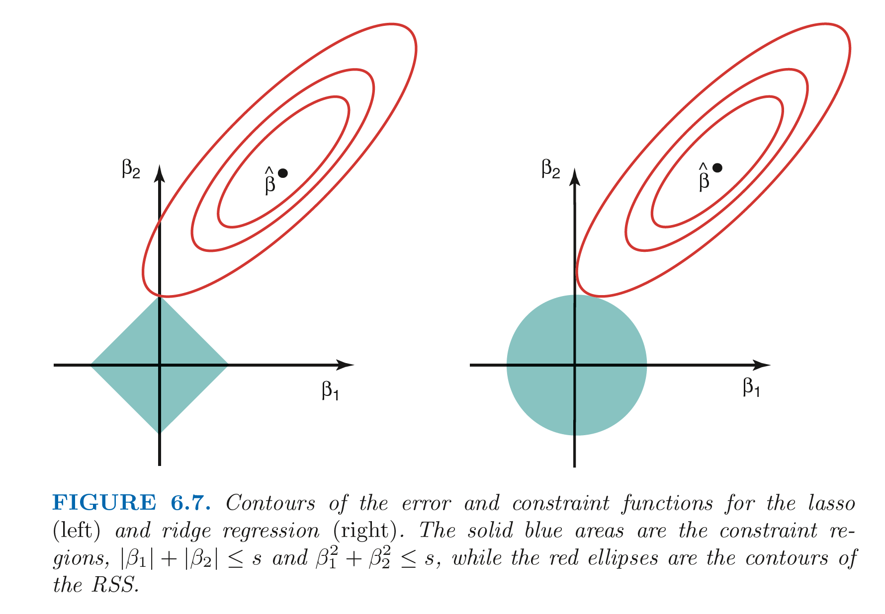
Above figure explains why estimated lasso coefficients can be 0. In the above figure, the least squares solution is marked as $\widehat{\beta}$ and the lasso and ridge regression constraints are marked as diamond and circle respectively. The ellipses that are centered around $\widehat{\beta}$ represents regions of constant RSS. As the ellipse expands away from least squares regression coefficient, RSS increases. The lasso and ridge regression coefficients are given by the points at which an ellipse contacts the region defined by the constraint. As the contour of ridge regression constraint does not have any sharp edges, an ellipse will never cross it at one of the axises and hence will never give a single 0 coefficient value. But, as the lasso constraint contour has corners at each of the axis, the ellipse will often intersect the constraint at one of the axes giving the 0 value for the coefficient.
Comparing the Lasso and Ridge Regression
Neither ridge regression nor the lasso will universally dominate the other. The lasso will perform better in the setting where a relatively samll number of predictors are statistically significant. If all the predictors have coefficients of equal magnitude, ridge regression will perform better. But the number of predictors that are related to the response is not known in advance, we need to cross-validate the model and then choose the best one.
Ridge regression shrinks every dimenion of the data by same proportion. Lasso shrinks every coefficient towards 0 by same amount and the smaller coefficients are shrinken all the way to 0.
Bayesian Interpretation for Ridge Regression and the Lasso
A Bayesian viewpoint of regression assumes that the coefficient vector $\beta$ has some prior distribution, $p(\beta)$. Then the likelihood of data can be represented as $f(Y \ | \ X, \beta)$. Multiplying the prior distribution from the likelihood gives us posterior distribution:
$$p(\beta | X,Y) \propto f(Y \ | \ X, \beta)\ p(\beta|X) = f(Y \ | \ X, \beta)\ p(\beta)$$
Let us assume that the prior distribution of $\beta$ is given by the density function $g$, then $p(\beta) = \prod_{j=1}^{p} g(\beta_j)$.
-
If $g$ is a Gaussian distribution with mean 0 and standard deviation some function of $\lambda$, the posterior mode of $\beta$ gives the ridge regression coefficient. The ridge regression coefficient is also the posterior mean.
-
If $g$ is a double exponential(Laplace) distribution with mean 0 and scale parameter some function of $\lambda$, the posterior mode of $\beta$ gives the lasso coefficient.
6.2.3 Selecting the Tuning Parameter
To design a better model, we need to select proper tuning parameter $\lambda$ or the constraint $s$. Cross-validation provides a concrete process to handle this. We can fit the models for different values of $\lambda$, and, by the process of cross-validation, select the best of it. Finally the model is fitted for the selected value of $\lambda$ using all the available observations.