Sometimes an experiment is designed in such a way that each item in one sample is paired with an item in the other. Let $D_1, D-2, …, D_n$ be a small random sample $(n \leq 30)$ of differences of the paired data. If the population of differences is approximately normal, the $100(1 - \alpha) %$ confidence interval for the mean difference $\mu_D$ is given as:
$$\overline{D} \pm t _{n-1, \alpha/2} \frac{s_D}{\sqrt{n}}$$
where $s_D$ is the sample standard deviation of $D_1, D_2, …, D_n$. If the sample size is large, the confidence interval is given as:
$$\overline{D} \pm z _{\alpha/2} \frac{s_D}{\sqrt{n}}$$
#### Confidence Intervals for the Variance and Standard Deviation of a Normal Population :Confidence interval for the population variance $\sigma^2$ (when the population is normal) is based on sample variance $s^2$ and a probability distribution known as chi-square distribution. To be more specific, if $X_1, X_2, …, X_n$ is a random sample from a normal population with variance $\sigma^2$, the sample variance can be given as:
$$s^2 = \frac{1}{n-1} \sum _{i=1}^{n} (X_i - \overline{X})^2$$
The quantity
$$\frac{(n-1)s^2}{\sigma^2} = \frac{\sum _{i=1}^{n} (X_i - \overline{X})^2}{\sigma^2}$$
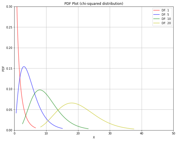
follows a chi-square distribution with degree of freedom $n-1$ and is denoted as $\chi _{n-1}^2$. The plot of chi-square distribution for various degree of freedoms is shown below. It should be noted that chi-square distribution are right-skewed and the value of chi-square statistic is always positive. Due to asymmetric nature of the chi-square distribution, the upper and lower conficence bound is computed by two different quantities. To find the upper and lower bounds for a $100(1 - \alpha) %$ confidence interval for a variance, the values that cut off areas of $\frac{\alpha}{2}$ in the right and left tails of the chi-square probability density curve are used. The calculation of confidence interval is shown by an example below.
from scipy.stats import chi2
import matplotlib.pyplot as plt

fig = plt.figure(figsize=(10,8))
ax = fig.add_subplot(111)

df=1
x = np.linspace(chi2.ppf(0.01, df), chi2.ppf(0.99, df), 1000)
ax.plot(x, chi2.pdf(x, df), 'r-', lw=2, alpha=0.6, label='DF: '+str(df))

df=5
x = np.linspace(chi2.ppf(0.01, df), chi2.ppf(0.99, df), 1000)
ax.plot(x, chi2.pdf(x, df), 'b-', lw=2, alpha=0.6, label='DF: '+str(df))

df=10
x = np.linspace(chi2.ppf(0.01, df), chi2.ppf(0.99, df), 1000)
ax.plot(x, chi2.pdf(x, df), 'g-', lw=2, alpha=0.6, label='DF: '+str(df))

df=20
x = np.linspace(chi2.ppf(0.01, df), chi2.ppf(0.99, df), 1000)
ax.plot(x, chi2.pdf(x, df), 'y-', lw=2, alpha=0.6, label='DF: '+str(df))

ax.set_ylim(0, 0.30)
ax.set_xlim(0, 50)
ax.set_xlabel('X')
ax.set_ylabel('PDF')
ax.set_title("PDF Plot (chi-squared distribution)")
ax.legend()
ax.grid()

plt.show()
Example: A simple random sample of 15 pistons is selected from a large population whose diameters are known to be normally distributed. The sample standard deviation of the piston diameters is s = 2.0 mm. Find a 95% confidence for the population variance $\sigma^2$ and population standard deviation $\sigma$.
Sol: The degree of freedom of chi-square distribution is $n-1 = 14$. From chi-square table, the upper and lower cut off points can be found as $\chi _{14, .975} = 5.63$ and $\chi _{14, .025} = 26.12$, i.e.
$$5.63 < \frac{(n-1)s^2}{\sigma^2} < 26.12$$
Solving this we get, $2.144 < \sigma^2 < 9.948$. The confidence interval for the population standard deviation $\sigma$ can be computed by taking the square root: $1.464 < \sigma < 3.154$.
The calculation of confidence interval based on chi-square distribution requires that the population is normal. If the population distribution deviates from normal, the calculated confidence interval can be misleading.
#### Prediction Intervals :A prediction interval is the interval that is likely to contain the value of an item sampled from a population at a future time. Let $\overline{X}$ be the sample mean of $n$ samples from a normally distributed population. It will have a normal distribution which can be given by $\overline{X} \sim N(\mu, \sigma^2/n)$. Suppose, at a future point, a value $Y$ is observed from the population. The distribution of $Y$ will be same as the population distribution, $Y \sim N(\mu, \sigma^2)$. Hence, the difference $Y - \overline{X}$ will be normally distributed with mean 0 and variance $\sigma^2(1 + 1/n)$. i.e.
$$\frac{Y - \overline{X}}{\sigma\sqrt{1 + 1/n}} \sim N(0, 1)$$
The population standard deviation $\sigma$ can be estimated as the sample standard deviation $s$ and hence the prediction interval can be given as:
$$\overline{X} \pm z _{\alpha/2} \times s\sqrt{1 + \frac{1}{n}}$$
For a smaller sample size, Student’s t distribution is used and the prediction interval can be given as:
$$\overline{X} \pm t _{n-1, \alpha/2} \times s\sqrt{1 + \frac{1}{n}}$$
One-sided prediction interval can be found similarly:
$$Lower \ bound = \overline{X} - t _{n-1, \alpha} \times s\sqrt{1 + \frac{1}{n}}$$
$$Upper \ bound = \overline{X} + t _{n-1, \alpha} \times s\sqrt{1 + \frac{1}{n}}$$
#### Reference :https://www.mheducation.com/highered/product/statistics-engineers-scientists-navidi/M0073401331.html