Applied
Q10. This question should be answered using the Weekly data set.
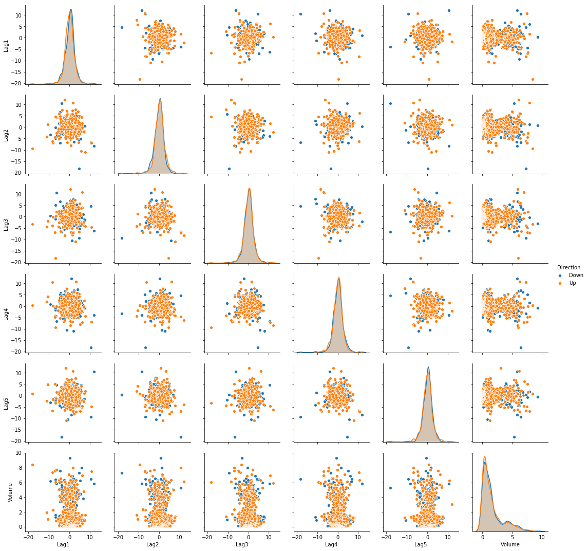
(a) Produce some numerical and graphical summaries of the Weekly data. Do there appear to be any patterns?
import seaborn as sns
weekly = pd.read_csv("data/Weekly.csv")

sns.pairplot(weekly, vars=['Lag1', 'Lag2', 'Lag3', 'Lag4', 'Lag5', 'Volume'], hue='Direction')
(b) Use the full data set to perform a logistic regression with Direction as the response and the five lag variables plus Volume as predictors. Use the summary function to print the results. Do any of the predictors appear to be statistically significant? If so, which ones?
Sol: Significant predictors are: Lag2
import statsmodels.api as sm
from statsmodels.discrete.discrete_model import Logit

weekly['trend'] = weekly['Direction'].map({'Down': 0, 'Up': 1})
X = weekly[['Lag1', 'Lag2', 'Lag3', 'Lag4', 'Lag5', 'Volume']]
X = sm.add_constant(X, prepend=True)
y = weekly['trend']

model = Logit(y, X)
result = model.fit()
print(result.summary())
Optimization terminated successfully.
         Current function value: 0.682441
         Iterations 4
                           Logit Regression Results
==============================================================================
Dep. Variable:                  trend   No. Observations:                 1089
Model:                          Logit   Df Residuals:                     1082
Method:                           MLE   Df Model:                            6
Date:                Mon, 10 Sep 2018   Pseudo R-squ.:                0.006580
Time:                        19:13:02   Log-Likelihood:                -743.18
converged:                       True   LL-Null:                       -748.10
                                        LLR p-value:                    0.1313
==============================================================================
                 coef    std err          z      P>|z|      [0.025      0.975]
------------------------------------------------------------------------------
const          0.2669      0.086      3.106      0.002       0.098       0.435
Lag1          -0.0413      0.026     -1.563      0.118      -0.093       0.010
Lag2           0.0584      0.027      2.175      0.030       0.006       0.111
Lag3          -0.0161      0.027     -0.602      0.547      -0.068       0.036
Lag4          -0.0278      0.026     -1.050      0.294      -0.080       0.024
Lag5          -0.0145      0.026     -0.549      0.583      -0.066       0.037
Volume        -0.0227      0.037     -0.616      0.538      -0.095       0.050
==============================================================================
(c) Compute the confusion matrix and overall fraction of correct predictions. Explain what the confusion matrix is telling you about the types of mistakes made by logistic regression.
Sol: The confusion matrix is shown below. The overall fraction of correct predictions is 56.11%. The model has higher flase positive rate.
print("\t\t Confusion Matrix")
print("\t Down  Up(Predicted)")
print("Down \t" + str(result.pred_table(threshold=0.5)[0]))
print("Up \t" + str(result.pred_table(threshold=0.5)[1]))
		 Confusion Matrix
	 Down  Up(Predicted)
Down 	[ 23. 418.]
Up 	[ 20. 524.]
(d) Now fit the logistic regression model using a training data period from 1990 to 2008, with Lag2 as the only predictor. Compute the confusion matrix and the overall fraction of correct predictions for the held out data (that is, the data from 2009 and 2010).
Sol: The confusion matrix is shown below. The overall fraction of correct predictions is 62.5%.
train = weekly.loc[weekly['Year'] <= 2008]
test = weekly.loc[weekly['Year'] >= 2009]

X = train[['Lag2']]
X = sm.add_constant(X, prepend=True)
y = train['trend']

model = Logit(y, X)
result = model.fit()
print(result.summary())
Optimization terminated successfully.
         Current function value: 0.685555
         Iterations 4
                           Logit Regression Results
==============================================================================
Dep. Variable:                  trend   No. Observations:                  985
Model:                          Logit   Df Residuals:                      983
Method:                           MLE   Df Model:                            1
Date:                Mon, 10 Sep 2018   Pseudo R-squ.:                0.003076
Time:                        19:53:30   Log-Likelihood:                -675.27
converged:                       True   LL-Null:                       -677.35
                                        LLR p-value:                   0.04123
==============================================================================
                 coef    std err          z      P>|z|      [0.025      0.975]
------------------------------------------------------------------------------
const          0.2033      0.064      3.162      0.002       0.077       0.329
Lag2           0.0581      0.029      2.024      0.043       0.002       0.114
==============================================================================
from sklearn.metrics import confusion_matrix

X_test = test[['Lag2']]
X_test = sm.add_constant(X_test, prepend=True)
y_test = test['trend']
predictions = result.predict(X_test) > 0.5

print("\t\t Confusion Matrix")
print("\t Down Up(Predicted)")
print("Down \t" + str(confusion_matrix(y_test, predictions)[0]))
print("Up \t" + str(confusion_matrix(y_test, predictions)[1]))
		 Confusion Matrix
	 Down Up(Predicted)
Down 	[ 9 34]
Up 	[ 5 56]
(e) Repeat (d) using LDA.
Sol: The confusion matrix is shown below. The overall fraction of correct predictions is 62.5%.
from sklearn.discriminant_analysis import LinearDiscriminantAnalysis
from sklearn.metrics import confusion_matrix

clf = LinearDiscriminantAnalysis()
clf.fit(train[['Lag2']], train['trend'])
y_predict = clf.predict(test[['Lag2']])

print("\t\t Confusion Matrix")
print("\t Down Up(Predicted)")
print("Down \t" + str(confusion_matrix(y_true=test['trend'], y_pred=y_predict)[0]))
print("Up \t" + str(confusion_matrix(y_true=test['trend'], y_pred=y_predict)[1]))
		 Confusion Matrix
	 Down Up(Predicted)
Down 	[ 9 34]
Up 	[ 5 56]
(f) Repeat (d) using QDA.
Sol: The confusion matrix is shown below. The overall fraction of correct predictions is 58.65%. The model always predict that the market will go up.
from sklearn.discriminant_analysis import QuadraticDiscriminantAnalysis

clf = QuadraticDiscriminantAnalysis()
clf.fit(train[['Lag2']], train['trend'])
y_predict = clf.predict(test[['Lag2']])

print("\t\t Confusion Matrix")
print("\t Down Up(Predicted)")
print("Down \t" + str(confusion_matrix(y_true=test['trend'], y_pred=y_predict)[0]))
print("Up \t" + str(confusion_matrix(y_true=test['trend'], y_pred=y_predict)[1]))
		 Confusion Matrix
	 Down Up(Predicted)
Down 	[ 0 43]
Up 	[ 0 61]
(g) Repeat (d) using KNN with K = 1.
Sol: The confusion matrix is shown below. The overall fraction of correct predictions is 49.04%.
from sklearn.neighbors import KNeighborsClassifier

neigh = KNeighborsClassifier(n_neighbors=1)
neigh.fit(train[['Lag2']], train['trend'])
y_predict = neigh.predict(test[['Lag2']])

print("\t\t Confusion Matrix")
print("\t Down Up(Predicted)")
print("Down \t" + str(confusion_matrix(y_true=test['trend'], y_pred=y_predict)[0]))
print("Up \t" + str(confusion_matrix(y_true=test['trend'], y_pred=y_predict)[1]))
		 Confusion Matrix
	 Down Up(Predicted)
Down 	[21 22]
Up 	[31 30]
(h) Which of these methods appears to provide the best results on this data?
Sol: The logistic regression and LDA have the minimum error rate.
Q11. In this problem, you will develop a model to predict whether a given car gets high or low gas mileage based on the Auto data set.
auto = pd.read_csv("data/Auto.csv")
auto.dropna(inplace=True)
auto = auto[auto['horsepower'] != '?']
auto['horsepower'] = auto['horsepower'].astype(int)
auto.head()
| mpg | cylinders | displacement | horsepower | weight | acceleration | year | origin | name | |
|---|---|---|---|---|---|---|---|---|---|
| 0 | 18.0 | 8 | 307.0 | 130 | 3504 | 12.0 | 70 | 1 | chevrolet chevelle malibu |
| 1 | 15.0 | 8 | 350.0 | 165 | 3693 | 11.5 | 70 | 1 | buick skylark 320 |
| 2 | 18.0 | 8 | 318.0 | 150 | 3436 | 11.0 | 70 | 1 | plymouth satellite |
| 3 | 16.0 | 8 | 304.0 | 150 | 3433 | 12.0 | 70 | 1 | amc rebel sst |
| 4 | 17.0 | 8 | 302.0 | 140 | 3449 | 10.5 | 70 | 1 | ford torino |
(a) Create a binary variable, mpg01, that contains a 1 if mpg contains a value above its median, and a 0 if mpg contains a value below its median.
auto['mpg01'] = np.where(auto['mpg']>=auto['mpg'].median(), 1, 0)
auto.head()
| mpg | cylinders | displacement | horsepower | weight | acceleration | year | origin | name | mpg01 | |
|---|---|---|---|---|---|---|---|---|---|---|
| 0 | 18.0 | 8 | 307.0 | 130 | 3504 | 12.0 | 70 | 1 | chevrolet chevelle malibu | 0 |
| 1 | 15.0 | 8 | 350.0 | 165 | 3693 | 11.5 | 70 | 1 | buick skylark 320 | 0 |
| 2 | 18.0 | 8 | 318.0 | 150 | 3436 | 11.0 | 70 | 1 | plymouth satellite | 0 |
| 3 | 16.0 | 8 | 304.0 | 150 | 3433 | 12.0 | 70 | 1 | amc rebel sst | 0 |
| 4 | 17.0 | 8 | 302.0 | 140 | 3449 | 10.5 | 70 | 1 | ford torino | 0 |
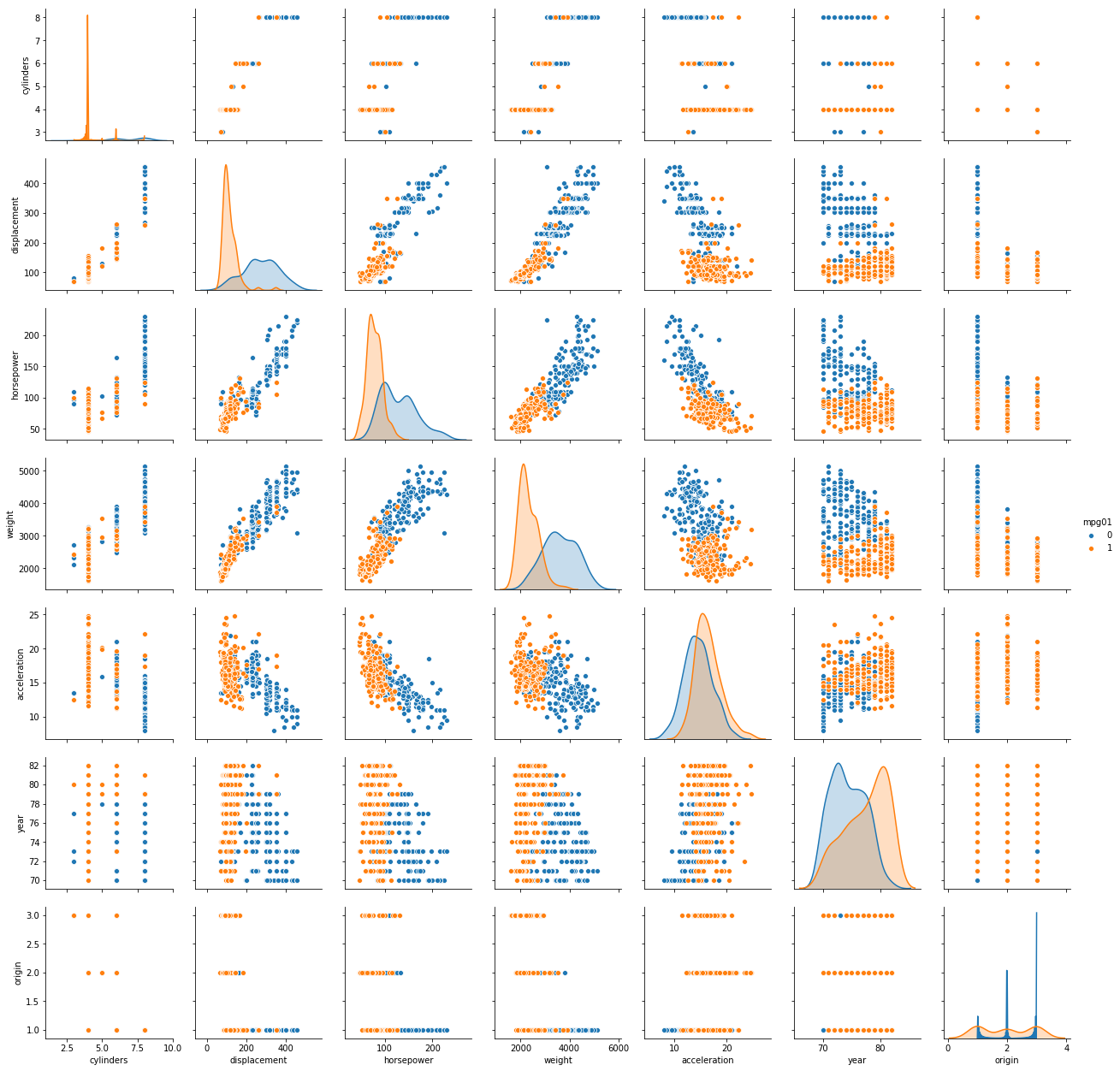
(b) Explore the data graphically in order to investigate the association between mpg01 and the other features. Which of the other features seem most likely to be useful in predicting mpg01? Scatterplots and boxplots may be useful tools to answer this question. Describe your findings.
Sol: The scatterplot of the data is shown below. As mpg01 with value 1 is shown with orange and value 0 is shown with blue, it is evident that certain combinations of predictors are present which can be used to model a classifier with high accuracy. For example, if we take a look at the scatter plot of weight and accelaration, it can be noted that the observations are decently segregated based on class.
sns.pairplot(auto, vars=['cylinders', 'displacement', 'horsepower', 'weight', 'acceleration',
                         'year', 'origin'], hue='mpg01')
(c) Split the data into a training set and a test set.
msk = np.random.rand(len(auto)) < 0.8
train = auto[msk]
test = auto[~msk]
print("Length of training data: " +str(len(train)))
print("Length of test data: " +str(len(test)))
Length of training data: 311
Length of test data: 81
(d) Perform LDA on the training data in order to predict mpg01 using the variables that seemed most associated with mpg01 in (b). What is the test error of the model obtained?
Sol: The test prediction accuracy for the model is 96.30%.
clf = LinearDiscriminantAnalysis()
clf.fit(train[['cylinders', 'displacement', 'horsepower', 'weight', 'acceleration', 'year']], train['mpg01'])
y_predict = clf.predict(test[['cylinders', 'displacement', 'horsepower', 'weight', 'acceleration', 'year']])

print("\t\t Confusion Matrix")
print("\t Down Up(Predicted)")
print("Down \t" + str(confusion_matrix(y_true=test['mpg01'], y_pred=y_predict)[0]))
print("Up \t" + str(confusion_matrix(y_true=test['mpg01'], y_pred=y_predict)[1]))
		 Confusion Matrix
	 Down Up(Predicted)
Down 	[32  3]
Up 	[ 0 46]
(e) Perform QDA on the training data in order to predict mpg01 using the variables that seemed most associated with mpg01 in (b). What is the test error of the model obtained?
Sol: The test prediction accuracy for the model is 97.53%.
clf = QuadraticDiscriminantAnalysis()
clf.fit(train[['cylinders', 'displacement', 'horsepower', 'weight', 'acceleration', 'year']], train['mpg01'])
y_predict = clf.predict(test[['cylinders', 'displacement', 'horsepower', 'weight', 'acceleration', 'year']])

print("\t\t Confusion Matrix")
print("\t Down Up(Predicted)")
print("Down \t" + str(confusion_matrix(y_true=test['mpg01'], y_pred=y_predict)[0]))
print("Up \t" + str(confusion_matrix(y_true=test['mpg01'], y_pred=y_predict)[1]))
		 Confusion Matrix
	 Down Up(Predicted)
Down 	[34  1]
Up 	[ 1 45]
(f) Perform logistic regression on the training data in order to predict mpg01 using the variables that seemed most associated with mpg01 in (b). What is the test error of the model obtained?
Sol: The test prediction accuracy for the model is 96.30%.
from sklearn.linear_model import LogisticRegression

clf = LogisticRegression()
clf.fit(train[['cylinders', 'displacement', 'horsepower', 'weight', 'acceleration', 'year']], train['mpg01'])
y_predict = clf.predict(test[['cylinders', 'displacement', 'horsepower', 'weight', 'acceleration', 'year']])

print("\t\t Confusion Matrix")
print("\t Down Up(Predicted)")
print("Down \t" + str(confusion_matrix(y_true=test['mpg01'], y_pred=y_predict)[0]))
print("Up \t" + str(confusion_matrix(y_true=test['mpg01'], y_pred=y_predict)[1]))
		 Confusion Matrix
	 Down Up(Predicted)
Down 	[34  1]
Up 	[ 2 44]
(g) Perform KNN on the training data, with several values of K, in order to predict mpg01. Use only the variables that seemed most associated with mpg01 in (b). What test errors do you obtain? Which value of K seems to perform the best on this data set?
Sol: The test prediction accuracy for the model is 96.30%. The optimal value of K is 20. On further increasing the value, no improvement is achieved.
K_values = [1, 2, 4, 8, 15, 20, 30, 50, 100]
for k in K_values:
    neigh = KNeighborsClassifier(n_neighbors=k)
    neigh.fit(train[['cylinders', 'displacement', 'horsepower', 'weight', 'acceleration', 'year']], train['mpg01'])
    y_predict = neigh.predict(test[['cylinders', 'displacement', 'horsepower', 'weight', 'acceleration', 'year']])

    print("\t\t Confusion Matrix for K = " +str(k))
    print("\t Down Up(Predicted)")
    print("Down \t" + str(confusion_matrix(y_true=test['mpg01'], y_pred=y_predict)[0]))
    print("Up \t" + str(confusion_matrix(y_true=test['mpg01'], y_pred=y_predict)[1]))
		 Confusion Matrix for K = 1
	 Down Up(Predicted)
Down 	[33  2]
Up 	[ 5 41]
		 Confusion Matrix for K = 2
	 Down Up(Predicted)
Down 	[34  1]
Up 	[ 6 40]
		 Confusion Matrix for K = 4
	 Down Up(Predicted)
Down 	[34  1]
Up 	[ 6 40]
		 Confusion Matrix for K = 8
	 Down Up(Predicted)
Down 	[34  1]
Up 	[ 2 44]
		 Confusion Matrix for K = 15
	 Down Up(Predicted)
Down 	[33  2]
Up 	[ 2 44]
		 Confusion Matrix for K = 20
	 Down Up(Predicted)
Down 	[33  2]
Up 	[ 1 45]
		 Confusion Matrix for K = 30
	 Down Up(Predicted)
Down 	[34  1]
Up 	[ 2 44]
		 Confusion Matrix for K = 50
	 Down Up(Predicted)
Down 	[34  1]
Up 	[ 2 44]
		 Confusion Matrix for K = 100
	 Down Up(Predicted)
Down 	[34  1]
Up 	[ 2 44]
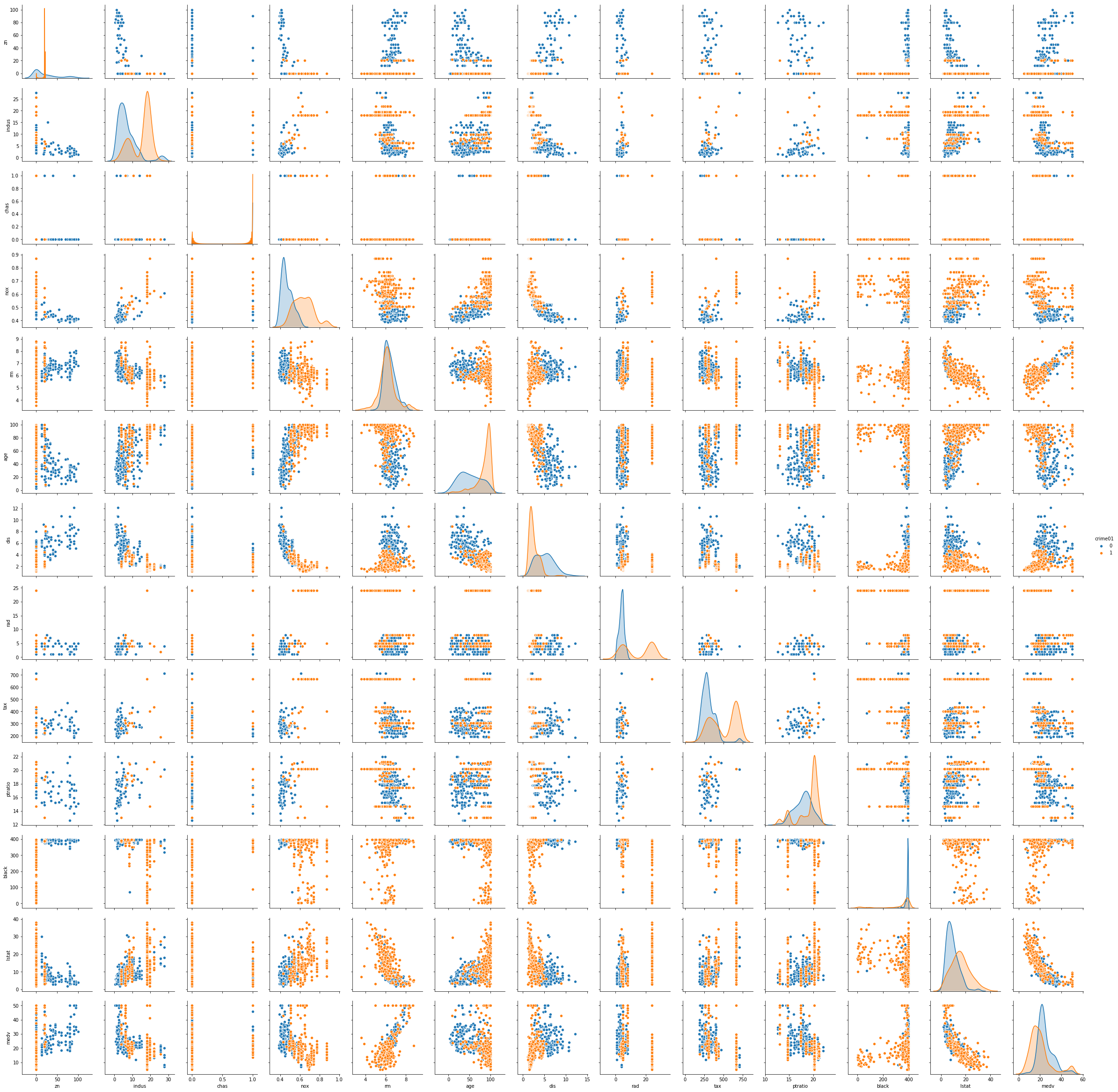
Q13. Using the Boston data set, fit classification models in order to predict whether a given suburb has a crime rate above or below the median. Explore logistic regression, LDA, and KNN models using various subsets of the predictors. Describe your findings.
Sol: From the scatterplot it is identified that the predictors that can be used to model the classifier are: ‘zn’, ‘chas’, ’nox’, ‘rm’, ‘age’, ‘dis’, ‘black’, ’lstat’, ‘medv’.
The test prediction accuracy for logistic regression is 81.48%. The test prediction accuracy for LDA is 81.48%. The test prediction accuracy for LDA is 77.78%. The test prediction accuracy for KNN (K=120) is 82.41%.
boston = pd.read_csv("data/Boston.csv")
boston['crime01'] = np.where(boston['crim']>=boston['crim'].median(), 1, 0)
boston.head()
| crim | zn | indus | chas | nox | rm | age | dis | rad | tax | ptratio | black | lstat | medv | crime01 | |
|---|---|---|---|---|---|---|---|---|---|---|---|---|---|---|---|
| 0 | 0.00632 | 18.0 | 2.31 | 0 | 0.538 | 6.575 | 65.2 | 4.0900 | 1 | 296 | 15.3 | 396.90 | 4.98 | 24.0 | 0 |
| 1 | 0.02731 | 0.0 | 7.07 | 0 | 0.469 | 6.421 | 78.9 | 4.9671 | 2 | 242 | 17.8 | 396.90 | 9.14 | 21.6 | 0 |
| 2 | 0.02729 | 0.0 | 7.07 | 0 | 0.469 | 7.185 | 61.1 | 4.9671 | 2 | 242 | 17.8 | 392.83 | 4.03 | 34.7 | 0 |
| 3 | 0.03237 | 0.0 | 2.18 | 0 | 0.458 | 6.998 | 45.8 | 6.0622 | 3 | 222 | 18.7 | 394.63 | 2.94 | 33.4 | 0 |
| 4 | 0.06905 | 0.0 | 2.18 | 0 | 0.458 | 7.147 | 54.2 | 6.0622 | 3 | 222 | 18.7 | 396.90 | 5.33 | 36.2 | 0 |
sns.pairplot(boston, vars=['zn', 'indus', 'chas', 'nox', 'rm',
                         'age', 'dis', 'rad', 'tax', 'ptratio', 'black', 'lstat', 'medv'], hue='crime01')
msk = np.random.rand(len(boston)) < 0.8
train = boston[msk]
test = boston[~msk]
print("Length of training data: " +str(len(train)))
print("Length of test data: " +str(len(test)))
Length of training data: 398
Length of test data: 108
clf = LogisticRegression()
clf.fit(train[['zn', 'chas', 'nox', 'rm', 'age', 'dis', 'black', 'lstat', 'medv']], train['crime01'])
y_predict = clf.predict(test[['zn', 'chas', 'nox', 'rm', 'age', 'dis', 'black', 'lstat', 'medv']])

print("\t\t Confusion Matrix")
print("\t Down Up(Predicted)")
print("Down \t" + str(confusion_matrix(y_true=test['crime01'], y_pred=y_predict)[0]))
print("Up \t" + str(confusion_matrix(y_true=test['crime01'], y_pred=y_predict)[1]))
		 Confusion Matrix
	 Down Up(Predicted)
Down 	[40  6]
Up 	[14 48]
clf = LinearDiscriminantAnalysis()
clf.fit(train[['zn', 'chas', 'nox', 'rm', 'age', 'dis', 'black', 'lstat', 'medv']], train['crime01'])
y_predict = clf.predict(test[['zn', 'chas', 'nox', 'rm', 'age', 'dis', 'black', 'lstat', 'medv']])

print("\t\t Confusion Matrix")
print("\t Down Up(Predicted)")
print("Down \t" + str(confusion_matrix(y_true=test['crime01'], y_pred=y_predict)[0]))
print("Up \t" + str(confusion_matrix(y_true=test['crime01'], y_pred=y_predict)[1]))
		 Confusion Matrix
	 Down Up(Predicted)
Down 	[43  3]
Up 	[17 45]
clf = QuadraticDiscriminantAnalysis()
clf.fit(train[['zn', 'chas', 'nox', 'rm', 'age', 'dis', 'black', 'lstat', 'medv']], train['crime01'])
y_predict = clf.predict(test[['zn', 'chas', 'nox', 'rm', 'age', 'dis', 'black', 'lstat', 'medv']])

print("\t\t Confusion Matrix")
print("\t Down Up(Predicted)")
print("Down \t" + str(confusion_matrix(y_true=test['crime01'], y_pred=y_predict)[0]))
print("Up \t" + str(confusion_matrix(y_true=test['crime01'], y_pred=y_predict)[1]))
		 Confusion Matrix
	 Down Up(Predicted)
Down 	[40  6]
Up 	[18 44]
K_values = [1, 2, 4, 8, 15, 20, 30, 50, 100, 120, 150]
for k in K_values:
    neigh = KNeighborsClassifier(n_neighbors=k)
    neigh.fit(train[['zn', 'chas', 'nox', 'rm', 'age', 'dis', 'black', 'lstat', 'medv']], train['crime01'])
    y_predict = neigh.predict(test[['zn', 'chas', 'nox', 'rm', 'age', 'dis', 'black', 'lstat', 'medv']])

    print("\t\t Confusion Matrix for K = " +str(k))
    print("\t Down Up(Predicted)")
    print("Down \t" + str(confusion_matrix(y_true=test['crime01'], y_pred=y_predict)[0]))
    print("Up \t" + str(confusion_matrix(y_true=test['crime01'], y_pred=y_predict)[1]))
		 Confusion Matrix for K = 1
	 Down Up(Predicted)
Down 	[40  6]
Up 	[17 45]
		 Confusion Matrix for K = 2
	 Down Up(Predicted)
Down 	[42  4]
Up 	[29 33]
		 Confusion Matrix for K = 4
	 Down Up(Predicted)
Down 	[42  4]
Up 	[22 40]
		 Confusion Matrix for K = 8
	 Down Up(Predicted)
Down 	[42  4]
Up 	[19 43]
		 Confusion Matrix for K = 15
	 Down Up(Predicted)
Down 	[41  5]
Up 	[19 43]
		 Confusion Matrix for K = 20
	 Down Up(Predicted)
Down 	[42  4]
Up 	[20 42]
		 Confusion Matrix for K = 30
	 Down Up(Predicted)
Down 	[43  3]
Up 	[17 45]
		 Confusion Matrix for K = 50
	 Down Up(Predicted)
Down 	[41  5]
Up 	[19 43]
		 Confusion Matrix for K = 100
	 Down Up(Predicted)
Down 	[38  8]
Up 	[12 50]
		 Confusion Matrix for K = 120
	 Down Up(Predicted)
Down 	[38  8]
Up 	[11 51]
		 Confusion Matrix for K = 150
	 Down Up(Predicted)
Down 	[38  8]
Up 	[12 50]