10.1 Graphs, Networks and Incidence Matrices:
Graphs consist of nodes and edges. For example, in the attached figure, the graph has $n=4$ nodes and $m=5$ edges. The graph can be interpreted as a circuit where nodes represent the points from which current flows and edges with the arrow represent the direction of its flow.
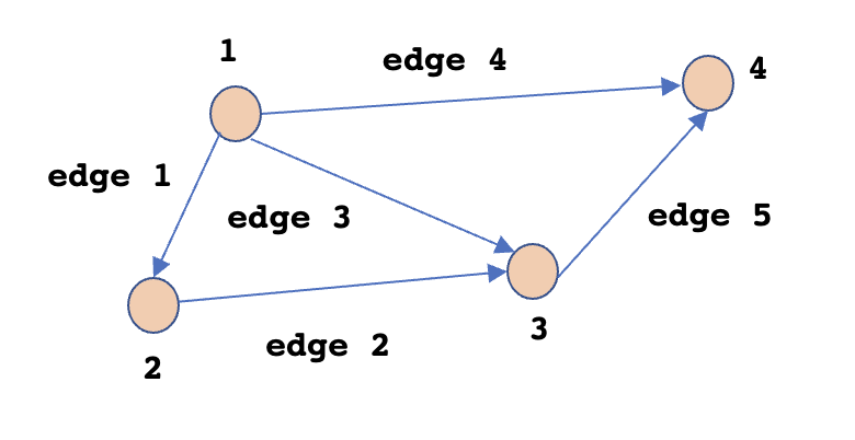
The above graph can be represented using a matrix, called as Incidence Matrix. The edges of the graph are represented using rows where entry at each column (one columnn for each of the node) index represents the start and end of the edge. An entry of $-1$ marks the start node of the edge and that of $1$ marks the end node of the edge. For example, $edge 1$ between node $1$ and $2$ can be represented by the row $\begin{bmatrix}-1 & 1 & 0 & 0\end{bmatrix}$. The overall Incidence Matrix where rows are numbered as per the edges is shown below.
$$\begin{align} A = \begin{bmatrix} -1 & 1 & 0 & 0 \\ 0 & -1 & 1 & 0 \\ -1 & 0 & 1 & 0 \\ -1 & 0 & 0 & 1 \\ 0 & 0 & -1 & 1 \end{bmatrix} \end{align}$$
The incidence matrix will have two non-zero entries for each of the rows. One interesting thing to note is the fact that edge $1,2,3$ forms a loop in the graphs. The rows in the incidence matrix representing these edges are dependent ($row3 = row2 + row1$).
10.1.1 Null Space of Incidence Matrix:
To find the null space of the incidence matrix, we have to solve the equation $Ax=0$. The vector x will be $\begin{bmatrix}x_1 & x_2 & x_3 & x_4\end{bmatrix}^T$. The entries $x_is$ can be viewed as the potentials at the nodes and the term $Ax$ is the potential difference between two of the nodes or potential difference across edges. The equation is given as:
$$\begin{align} \begin{bmatrix} -1 & 1 & 0 & 0 \\ 0 & -1 & 1 & 0 \\ -1 & 0 & 1 & 0 \\ -1 & 0 & 0 & 1 \\ 0 & 0 & -1 & 1 \end{bmatrix} \begin{bmatrix} x_1 \\ x_2 \\ x_3 \\ x_4 \end{bmatrix} = \begin{bmatrix} 0 \\ 0 \\ 0 \\ 0 \\ 0 \end{bmatrix} \implies \begin{bmatrix} x_2 - x_1 \\ x_3 - x_2 \\ x_3 - x_1 \\ x_4 - x_1 \\ x_4 - x_3 \end{bmatrix} = \begin{bmatrix} 0 \\ 0 \\ 0 \\ 0 \\ 0 \end{bmatrix} \end{align}$$
This gives us $c\begin{bmatrix} 1 \\ 1 \\ 1 \\ 1 \end{bmatrix}$ as the basis for the null space, i.e. $dim(N(A)) = 1$.
10.1.2 Column Space of Incidence Matrix:
Another way to form the incidence matrix is by grounding one of the nodes (making its potential 0). This gives us an incidence matrix just with $3$ columns which will be independent of each other. This makes the basis of column space a 3-dimensional subspace giving the rank of the incidence matrix $A$ as $3(rank(A)=3)$.
10.1.3 Left Null Space of Incidence Matrix:
Left Null Space (Null Space of $A^T$) of incidence matrix $A$ can be obtained by solving the equation $A^Ty=0$. The equation $A^Ty=0$ is shown below. The dimension of Left Null Space is $dim((N(A^T)) = m-r=5-3=2$. This also depicts total number of loops in the graph. The vector $\begin{bmatrix}y_1 & y_2 & y_3 & y_4 & y_5\end{bmatrix}^T$ can be viewed as the currents flowing through each of the edges.
$$\begin{align} \begin{bmatrix} -1 & 0 & -1 & -1 & 0 \\ 1 & -1 & 0 & 0 & 0 \\ 0 & 1 & 1 & 0 & -1 \\ 0 & 0 & 0 & 1 & 1 \end{bmatrix} \begin{bmatrix} y_1 \\ y_2 \\ y_3 \\ y_4 \\ y_5 \end{bmatrix} = \begin{bmatrix} 0 \\ 0 \\ 0 \\ 0 \end{bmatrix} \end{align}$$
First equation for the above matrix equation is: $-y_1 - y_3 - y_4 = 0$. This indicates the net current flowing through node $1$ is 0, i.e. the charge doesn’t accumulate at this node.
10.1.4 Row Space of Incidence Matrix:
The dimension of row space of the incidence matrix is $3 (rank = 3)$. Row Space can be defined as the column sapce of $A^T$, i.e $C(A^T)$.
$$\begin{align} A^T = \begin{bmatrix} -1 & 0 & -1 & -1 & 0 \\ 1 & -1 & 0 & 0 & 0 \\ 0 & 1 & 1 & 0 & -1 \\ 0 & 0 & 0 & 1 & 1 \end{bmatrix} \end{align}$$
If we look closely, $col3 = col1 + col2$ and $col5 = col4 - col1 - col2$ for $A^T$. This means $col1, col2, col4$ are independent and they form the basis for $C(A^T)$. These columns corresponds to the rows of $A$, i.e. the edges of the graphs. These edges are $edge1, edge2, edge4$. The graph formed using these edges has all the nodes and edges but with the edges forming the loops removed, i.e. they form a graph without a loop (which can also be called as tree).
10.1.5 Conclusion:
-
The number of loops in the graph is given by $dim(N(A^T)) = m - r$, where $r=rank=n-1$. i.e. $loops = edges - (nodes - 1)$. This formula can be restructured as: $nodes - edges + loops = 1$. This is called as Euler’s Formula.
-
As $Ax$ represents the potentail difference across the edges and $y$ represents the current through them, with a resistance of $C$, the equation for Ohm’s law can be given as $y=CAx$. The term $A^Ty$ depicts the current flowing through the circuit. If we supply an external current $f$, the overall representation is: $A^TCAx=f$.