2.1 Means and averages
Mean of a sample is a summary statistics that can be computed as (where n is the total number of samples): $$\mu = \frac{1}{n} \sum_i{x_i}$$ An average is one of many summary statistics that can be used to describe the typical value or the central tendency of a sample.
2.2 Variance
As mean describes the central tendency of a sample, Variance is intended to describe the spread. The variance is defined as: $$\sigma^2 = \frac{1}{n} \sum_i{(x_i-\mu)^2}$$ The square root of variance is Standard Deviation. Sample variance, which is used to estimate the variance of a population can be computed by having n-1 in the denominator as follows: $$s^2 = \frac{1}{n-1} \sum_i{(x_i-\mu)^2}$$
2.3 Distributions
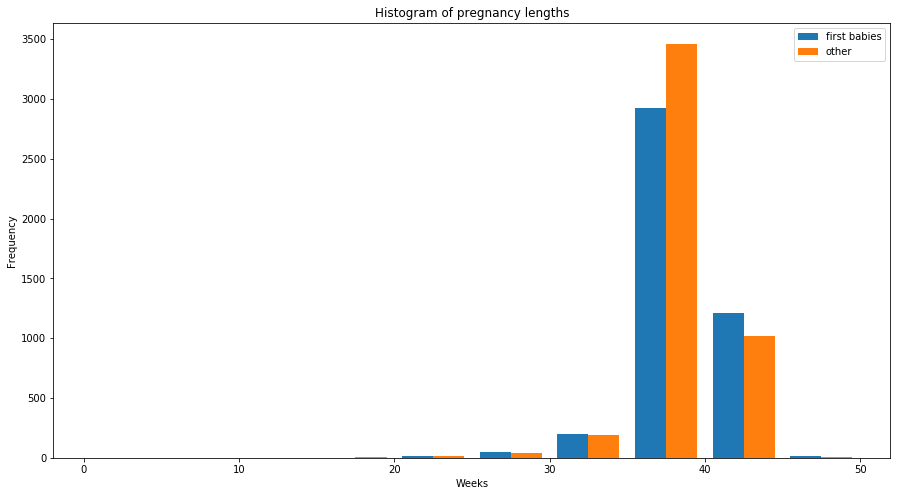
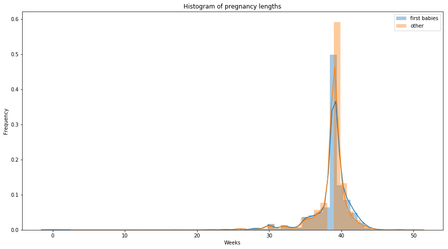
The most common representation of a distribution is a histogram, which is a graph that shows the frequency or probability of each value. Frequency means the number of times a value appears in the dataset and probability is frequency divided by the sample size. Usually histogram is the plot of frequencies. Normalized histogram, which is the plot of probabilities is called PMF (Probability Mass Function). PMFs are generally used to describe discrete random variables/ categorical variables. Histogram plot and PMF of pregnancy lengths for first babies and othres is shown below.
Histograms are not useful for comparing two distributions as some of the apparent difference in histogram may arise due to sample sizes. PMF solves this problem.
import pandas as pd
# Reference to extract the columns: http://greenteapress.com/thinkstats/survey.py
pregnancies = pd.read_fwf("2002FemPreg.dat",
                         names=["caseid", "nbrnaliv", "babysex", "birthwgt_lb",
                               "birthwgt_oz", "prglength", "outcome", "birthord",
                               "agepreg", "finalwgt"],
                         colspecs=[(0, 12), (21, 22), (55, 56), (57, 58), (58, 60),
                                (274, 276), (276, 277), (278, 279), (283, 285), (422, 439)])
import matplotlib.pyplot as plt
import seaborn as sns
first_child = pregnancies[(pregnancies['outcome'] == 1) & (pregnancies['birthord'] == 1)]['prglength']
other = pregnancies[(pregnancies['outcome'] == 1) & (pregnancies['birthord'] != 1)]['prglength']
fig = plt.figure(figsize=(15, 8))
ax = fig.add_subplot(111)
plt.hist([first_child, other],label=['first babies', 'other'])
ax.set_xlabel('Weeks')
ax.set_ylabel('Frequency')
ax.set_title('Histogram of pregnancy lengths')
plt.legend()
plt.show()

fig = plt.figure(figsize=(15, 8))
ax = fig.add_subplot(111)
sns.distplot(first_child, label='first babies')
sns.distplot(other, label='other')
ax.set_xlabel('Weeks')
ax.set_ylabel('Frequency')
ax.set_title('Histogram of pregnancy lengths')
plt.legend()
plt.show()
2.6 Representing PMFs
Mean and Variance can be computed from PMF as follows (where ps are the corresponding probabilities of xs): $$\mu = \frac{1}{n} \sum_i{p_ix_i}$$ $$\sigma^2 = \frac{1}{n-1} \sum_i{p_i(x_i-\mu)^2}$$
PMFs can be shown by line plot when sample size is large.
2.8 Outliers
Outliers are values that are far from the central tendency. Outliers might be caused by errors in collecting or processing the data, or they might be correct but unusual measurements. It is always a good idea to check for outliers, and sometimes it is useful and appropriate to discard them.