The Mistake That Makes Gradient Descent Work

Machine learning starts with a simple idea: find the model that makes the fewest mistakes. We measure those mistakes with a loss function, and training is the process of driving that loss downward. The natural conclusion is that we should keep descending until we reach the lowest possible point—the deepest valley in the landscape.

There is a problem with this idea. The deepest valley is not always the best place to be.

A model can fit its training data extraordinarily well and still perform badly on examples it has never seen. In fact, the solution with the lowest possible training loss can sometimes be less useful than a solution that makes slightly more mistakes on the training data but behaves more reliably on new data. The best fit on paper is not necessarily the best fit in the real world.

This is why machine learning has accumulated so many ways of resisting overfitting. We add penalties to the objective, stop training before the model has a chance to memorize too much, inject noise, constrain the parameters, and use a variety of other techniques to keep the model from becoming too attached to the peculiarities of its training set. These are deliberate interventions. We add them because we know that fitting the training data too perfectly can be dangerous.

But there is another form of regularization hiding in plain sight.

The optimization algorithm we use to train models already has a preference for certain kinds of solutions. Gradient descent tends to avoid some minima and settle into others. Nobody has to explicitly tell it to prefer broad, forgiving valleys over narrow, brittle ones. The preference emerges from a limitation that seems almost trivial: a computer cannot move continuously. It has to take steps.

To understand why that matters, imagine the loss function as a landscape of hills and valleys and the model as a walker trying to get downhill. At every point, the walker looks at the slope beneath its feet and chooses the direction that takes it downward most quickly.

In an ideal mathematical world, the walker would not really need to take steps. It could flow continuously down the landscape, constantly adjusting its direction as the ground changed beneath it. Every tiny change in the terrain would immediately influence its motion. There would be no hesitation and no commitment to a direction beyond the instant in which that direction was correct.

A computer cannot do this. It has to work in discrete moves. It looks at the slope where it is standing, decides how large a step to take, moves, and then looks again. Each step is therefore based on a small assumption: that the terrain will not change too dramatically between where the walker is now and where it lands next.

Usually, that assumption is good enough. But landscapes are not equally well behaved everywhere.

Consider a broad, gently curved valley. As the walker moves, the slope changes gradually. A step taken in the direction that looks downhill now will still be a sensible step a moment later. Even if the walker does not account for every subtle change in the terrain, it will tend to make steady progress toward the bottom.

Now imagine a narrow valley with steep walls. The situation changes completely. The walker looks downhill and commits to a step, but the ground curves sharply underneath it. By the time the walker reaches the end of the step, the direction that was correct at the beginning may no longer be correct. Instead of arriving neatly at the bottom, the walker overshoots it and starts climbing the opposite wall. The next step sends it back in the other direction, and the process can continue.

The sharper the valley, the more severe the problem. A narrow valley can keep throwing the walker from one side to the other. A broad valley gives it room to settle.

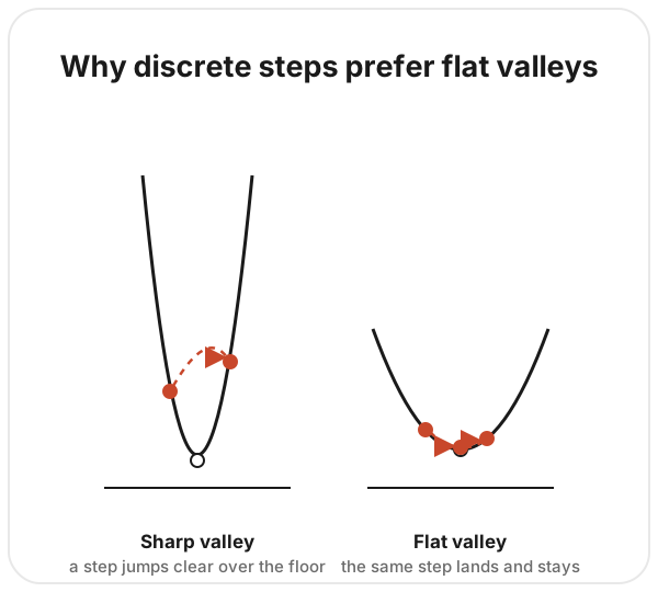
This creates an interesting bias. Gradient descent is not equally comfortable everywhere in the loss landscape. Sharp regions are difficult to settle into because finite steps can carry the optimizer straight through them. Flatter regions are more forgiving. The optimizer can move into them without constantly being kicked back out.

Given enough time, this means that discrete gradient descent naturally tends to favor wider, flatter regions of the landscape.

That matters because a flat minimum is usually a more forgiving solution. Imagine slightly disturbing the parameters of a model. If the model is sitting in a sharp minimum, even a small change can cause its loss to rise dramatically. The solution works well at one very specific point, but there is little room for error. A flat minimum is different. There is a whole neighborhood around the solution where the loss remains low. Small changes do not immediately destroy the model’s performance.

That does not mean that every flat minimum generalizes well or that every sharp minimum is bad. The relationship between flatness and generalization is more subtle than that. But the intuition is useful: a solution with room around it is generally less brittle than one that works only at a single, precise configuration.

And this is where the apparent flaw in gradient descent becomes interesting.

Its inability to follow the landscape perfectly is not simply a weakness of numerical computation. The fact that it takes finite steps changes what the optimizer tends to settle into. The same oversized step that makes it difficult to remain trapped in a narrow valley can make it easier to settle into a broader one.

In other words, the optimizer’s clumsiness becomes a kind of filter.

The effect is not merely something we can observe in a picture. We can make it precise by comparing the path taken by ordinary gradient descent with the path that an ideal, continuously moving optimizer would take. Once we do that, something surprising appears: the difference between the two paths has a structure. The discrete optimizer behaves, to a good approximation, as though it were solving a slightly different optimization problem.

That modified problem contains the original loss plus an additional penalty. The penalty becomes larger in regions where the landscape is steep and smaller in regions where it is flat. The optimizer therefore behaves as though it has been given an extra reason to move away from sharply curved regions and toward broader ones.

No one had to add this penalty.

It appears simply because the machine takes steps.

This is what is meant by implicit regularization. We normally think of regularization as something we consciously introduce into a model: a penalty, a constraint, early stopping, noise, or some other intervention designed to prevent overfitting. Here, the regularization is already present in the optimization procedure itself. It is a consequence of the gap between the smooth mathematical process we imagine and the discrete process the computer actually performs.

There is something satisfying about that.

We often think of numerical approximations as compromises. The mathematics says one thing; the computer gives us an approximation because it cannot reproduce the ideal exactly. Yet in this case, the approximation is doing useful work. The optimizer’s inability to move perfectly through the landscape makes some solutions harder to inhabit than others.

Gradient descent works, in part, because it does not behave exactly as the mathematical ideal says it should.

The mistake is the feature.

---

Appendix: Where the Penalty Comes From

The mathematical difference between continuous gradient flow and discrete gradient descent can be exposed with a Taylor expansion. The idea is simple: describe where a continuously moving parameter vector will be after a short interval, including not only its current direction of motion but also how that direction is changing. Then compare that prediction with the actual step made by gradient descent.

In continuous gradient flow, the parameters \(\phi\) move in the direction of the negative gradient of the loss \(L\):

\[ \frac{d\phi(t)}{dt} = -\nabla L(\phi(t)). \]

Expanding the trajectory a short time \(\Delta t\) into the future with a Taylor expansion gives

\[ \phi(t + \Delta t) = \phi(t) + \Delta t\,\frac{d\phi}{dt} + \frac{(\Delta t)^2}{2}\,\frac{d^2\phi}{dt^2} + \mathcal{O}\big((\Delta t)^3\big). \]

The second derivative follows from the chain rule:

\[ \frac{d^2\phi}{dt^2} = \frac{d}{dt}\big(-\nabla L(\phi)\big) = -\nabla^2 L(\phi)\,\frac{d\phi}{dt} = \nabla^2 L(\phi)\,\nabla L(\phi). \]

Substituting this into the expansion gives

\[ \phi(t + \Delta t) = \phi(t) - \Delta t\,\nabla L(\phi) + \frac{(\Delta t)^2}{2} \nabla^2 L(\phi)\,\nabla L(\phi) + \mathcal{O}\big((\Delta t)^3\big). \]

Gradient descent, however, uses the discrete update

\[ \phi_{k+1} = \phi_k - \alpha\,\nabla L(\phi_k), \]

where \(\alpha\) is the learning rate. Treating one gradient-descent step as a time interval of length \(\alpha\), the discrete trajectory is simply

\[ \phi(t+\alpha) = \phi(t) - \alpha\,\nabla L(\phi). \]

The continuous trajectory therefore contains an additional second-order term involving the curvature of the loss surface, while the discrete update does not. The difference between the two is approximately

\[ \text{drift} \approx -\frac{\alpha^2}{2}\, \nabla^2 L(\phi)\,\nabla L(\phi). \]

The next step is to ask whether we can find a modified loss whose continuous gradient flow reproduces the behavior of the discrete update.

Suppose that modified loss has the form

\[ \widetilde{L}(\phi) = L(\phi) + \alpha R(\phi). \]

Its gradient flow is then

\[ \frac{d\phi}{dt} = -\nabla\widetilde{L} = -\nabla L(\phi) - \alpha\,\nabla R(\phi). \]

Now expand this trajectory to second order in \(\alpha\):

\[ \phi(t + \alpha) \approx \phi(t) - \alpha\,\nabla L(\phi) - \alpha^2\,\nabla R(\phi) + \frac{\alpha^2}{2}\, \nabla^2 L(\phi)\,\nabla L(\phi). \]

We want this to match the actual discrete step,

\[ \phi(t+\alpha) = \phi(t) - \alpha\nabla L(\phi). \]

The first-order terms already agree, so the second-order terms must cancel:

\[ -\alpha^2\,\nabla R(\phi) + \frac{\alpha^2}{2}\, \nabla^2 L(\phi)\,\nabla L(\phi) = 0. \]

Therefore,

\[ \nabla R(\phi) = \frac{1}{2}\, \nabla^2 L(\phi)\,\nabla L(\phi). \]

We can use the identity

\[ \nabla \left( \frac{1}{2}\|\nabla L(\phi)\|^2 \right) = \nabla^2 L(\phi)\,\nabla L(\phi), \]

which means

\[ \nabla R(\phi) = \frac{1}{4} \nabla \left( \|\nabla L(\phi)\|^2 \right). \]

Integrating gives

\[ R(\phi) = \frac{1}{4} \|\nabla L(\phi)\|^2. \]

Substituting this into the modified objective gives

\[ \boxed{ \widetilde{L}_{\mathrm{GD}}[\phi] = L[\phi] + \frac{\alpha}{4} \|\nabla L(\phi)\|^2 } \]

The result is the hidden regularizer. To this order, discrete gradient descent behaves as though the original loss had been augmented by a term proportional to the squared gradient magnitude. Where the landscape is steep, this additional cost is larger; where the landscape is flat, it becomes smaller. The mathematics therefore reproduces the intuition from the main text: discrete steps create a bias away from sharply varying regions and toward flatter ones.

There is one subtle point worth emphasizing. It is easy to arrive at a negative sign for the correction if the modified flow is expanded only to first order. That truncation is inconsistent with the calculation because the effect we are trying to capture first appears at second order. Dropping the curvature term from the modified trajectory changes the matching and flips the sign. Keeping both trajectories to the same order produces the positive correction above, which is consistent with the geometric picture: the additional term penalizes steep regions rather than rewarding them.

The important point is not merely that such a correction can be written down. It is that the correction is generated by the discretization itself. There is no additional line of code and no explicitly chosen regularization coefficient responsible for it. The optimizer’s finite step is enough.